
Gates, the gating strategy, and reading the numbers#
A gate is a named region in one or two dimensions plus the display scaling its boundary was drawn on. That last part is not decoration: the same vertices mean different populations on a linear and a logicle axis, so a gate that does not carry its transform cannot be re-applied, saved or shared honestly.
What a cytometrist actually has, though, is not a gate but a strategy:
debris, then singlets, then live, then lineage — each step evaluated only on the
events its parent kept. ov.flow models that tree as an object that belongs to
the analysis rather than to any one sample, which is what makes applying one
strategy to ninety files possible.
This notebook continues from reading and compensation.
# No data of your own is needed. ov.datasets.flow_demo_fcs() writes a SIMULATED
# FCS 3.1 file into the current working directory: 59,600 events, nine known
# populations, a real $SPILLOVER keyword, and a detector noise floor that pushes
# dim events below zero — which is why a log display axis will not do.
import numpy as np, pathlib
import omicverse as ov

ov.style()          # omicverse's plotting defaults — call this once, up front

path = ov.datasets.flow_demo_fcs()
print(path)
🔬 Starting plot initialization...
🧬 Detecting GPU devices…
✅ Apple Silicon MPS detected
    • [MPS] Apple Silicon GPU - Metal Performance Shaders available

   ____            _     _    __
  / __ \____ ___  (_)___| |  / /__  _____________
 / / / / __ `__ \/ / ___/ | / / _ \/ ___/ ___/ _ \
/ /_/ / / / / / / / /__ | |/ /  __/ /  (__  )  __/
\____/_/ /_/ /_/_/\___/ |___/\___/_/  /____/\___/

🔖 Version: 2.2.4   📚 Tutorials: https://omicverse.readthedocs.io/
✅ plot_set complete.

flow_demo.fcs
import omicverse as ov
import matplotlib.pyplot as plt
import numpy as np

adata = ov.datasets.flow_demo()      # = read_fcs(flow_demo_fcs()) + obs['population']
ov.flow.compensate(adata)

lin = ov.flow.Linear(t=262144.0)
lg  = ov.flow.Logicle(t=262144.0, m=4.5, w=1.0, a=0.0)
adata
AnnData object with n_obs × n_vars = 59600 × 8
    obs: 'sample', 'population'
    var: 'n', 'channel', 'marker', 'PnB', 'PnE', 'PnG', 'PnR'
    uns: 'meta', 'fcs', 'flow_demo', 'flow'
    layers: 'uncompensated'
Gate geometry#
Five kinds, following Gating-ML 2.0 so they round-trip through the interchange format without a second representation:
Gate |
What it is |
|---|---|
|
axis-aligned interval in 1..n dims; |
|
arbitrary 2-D region — the gate people actually draw |
|
Mahalanobis region, parameterised by covariance and squared distance |
|
one divider per dimension → 2ⁿ populations that share their dividers |
|
AND / OR / NOT over populations already computed |
Note at(600) below. A threshold is a data value — 600 units of CD3 — and
writing it as the scale-space number it happens to equal is how a gate silently
drifts when the transform is retuned.
def at(v):
    """A data value expressed on the logicle scale — how a threshold is really
    written. Typing 0.42 instead of at(600) is how gates drift."""
    return float(lg.apply(np.array([float(v)]))[0])

cells = ov.flow.PolygonGate(
    name="Cells", dims=("FSC-A", "SSC-A"),
    transforms={"FSC-A": lin, "SSC-A": lin},
    vertices=np.array([[0.12,0.01],[0.12,0.17],[0.40,0.32],
                       [0.68,0.32],[0.68,0.09],[0.38,0.01]]))
singlets = ov.flow.PolygonGate(
    name="Singlets", dims=("FSC-A", "FSC-H"),
    transforms={"FSC-A": lin, "FSC-H": lin},
    vertices=np.array([[0.05,0.03],[0.05,0.10],[0.75,0.86],[0.75,0.69]]))
live = ov.flow.RectangleGate(
    name="Live", dims=("Viability",), transforms={"Viability": lg},
    bounds=((None, at(1200)),))
cd3 = ov.flow.RectangleGate(
    name="CD3+", dims=("CD3",), transforms={"CD3": lg},
    bounds=((at(600), None),))
quad = ov.flow.QuadrantGate(
    name="CD4/CD8", dims=("CD4", "CD8"), transforms={"CD4": lg, "CD8": lg},
    dividers=(at(600), at(600)),
    quadrant_names=("DN", "CD4+CD8-", "CD4-CD8+", "DP"))

gs = ov.flow.GatingStrategy("T cell panel")
gs.add_gate(cells)
gs.add_gate(singlets, parent="Cells")
gs.add_gate(live,     parent="Singlets")
gs.add_gate(cd3,      parent="Live")
gs.add_gate(quad,     parent="CD3+")
print(gs.tree())
root
  └ Cells
    └ Singlets
      └ Live
        └ CD3+
          └ CD4/CD8
          └ DN
          └ CD4+CD8-
          └ CD4-CD8+
          └ DP
Applying the strategy#
apply walks the tree, evaluating each gate only on the events its parent
kept, and writes one boolean column per population into obs.
res = gs.apply(adata)
res.stats()
  population    parent  count  parent_count  freq_parent  freq_total  low_n
0       CD3+      Live  28895         41574     0.695026    0.484815  False
1   CD4+CD8-      CD3+  16999         28895     0.588302    0.285218  False
2   CD4-CD8+      CD3+   9998         28895     0.346011    0.167752  False
3    CD4/CD8      CD3+  28895         28895     1.000000    0.484815  False
4      Cells      root  48587         59600     0.815218    0.815218  False
5         DN      CD3+   1398         28895     0.048382    0.023456  False
6         DP      CD3+    500         28895     0.017304    0.008389  False
7       Live  Singlets  41574         44785     0.928302    0.697550  False
8   Singlets     Cells  44785         48587     0.921749    0.751426  False
freq_parent is the number people actually report — “58.8% of CD3+” —
and it is meaningless without its denominator, so the parent is named in its own
column instead of being left implicit.
low_n flags populations small enough that the percentage is noise: a frequency
quoted off 30 events has a 95% confidence interval of roughly ±18 points, and
printing it to one decimal place, as every cytometry tool does, is false
precision.
Seeing the gates#
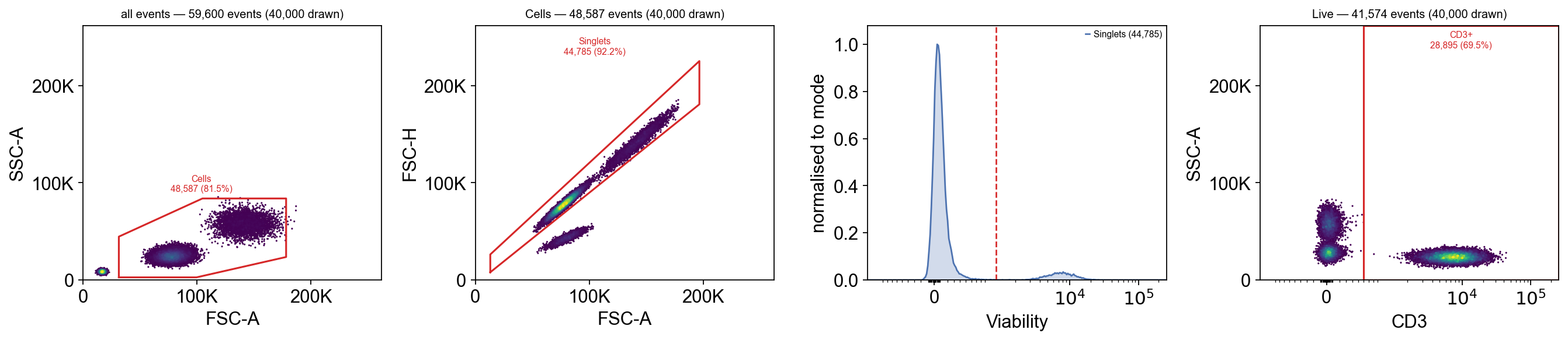
Here is the sequence. Each panel is drawn on its parent’s events, which is what makes a hierarchy readable — and each gate is drawn in the transform it carries, so the boundary cannot disagree with the mask.
fig, axes = plt.subplots(1, 4, figsize=(17, 3.9))

ov.flow.biaxial(adata, "FSC-A", "SSC-A", gates=[cells], result=res,
                ax=axes[0], max_events=40000)
ov.flow.biaxial(adata, "FSC-A", "FSC-H", gates=[singlets], result=res,
                population="Cells", ax=axes[1], max_events=40000)
ov.flow.histogram(adata, "Viability", gates=[live], result=res,
                  populations=["Singlets"], ax=axes[2])
ov.flow.biaxial(adata, "CD3", "SSC-A", gates=[cd3],
                transforms={"CD3": lg, "SSC-A": lin}, result=res,
                population="Live", ax=axes[3], max_events=40000)
plt.tight_layout()
Does the singlet gate exclude anything?#
A worthwhile question to ask of any gate, and one the picture answers only approximately. Doublets have roughly the same pulse area as singlets but a much lower pulse height, so they fall below the FSC-A ≈ FSC-H diagonal. Since this sample is synthetic we can check the gate against the truth:
kept    = adata.obs["population"].to_numpy()[res.masks["Singlets"]]
n_in    = int((kept == "doublet").sum())
n_total = int((adata.obs["population"] == "doublet").sum())
print(f"doublets in the singlet gate: {n_in:,} of {n_total:,} "
      f"({n_in / n_total:.1%})")
doublets in the singlet gate: 0 of 3,800 (0.0%)
The quadrant#
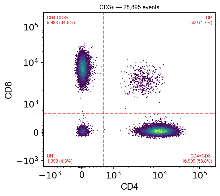
A quadrant gate is one gate with several outputs, not four rectangles: the quadrants share their dividers, so moving a divider must move every boundary at once. Four independent gates drift apart the first time someone edits one.
The four corner percentages are the entire point of the plot.
ov.flow.biaxial(adata, "CD4", "CD8", gates=[quad], result=res,
                population="CD3+", figsize=(4.8, 4.4), max_events=40000)
None
The hierarchy#
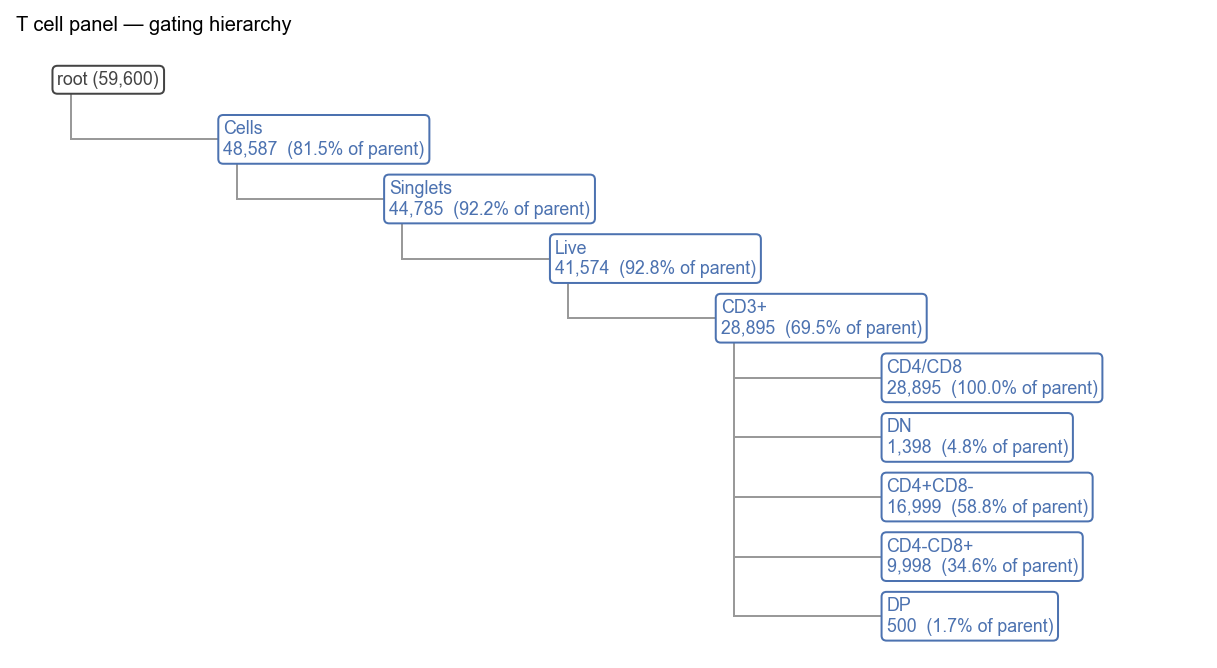
gs.tree() prints the same shape as text, which is better in a terminal. The
drawn version carries the numbers, and that is what a reader checks: a
population that keeps 3% of its parent where you expected 60% is obvious here
and invisible in a sorted table. Nodes below min_events are flagged.
ov.flow.hierarchy(gs, result=res, figsize=(9.5, 5))
None
Back-gating#
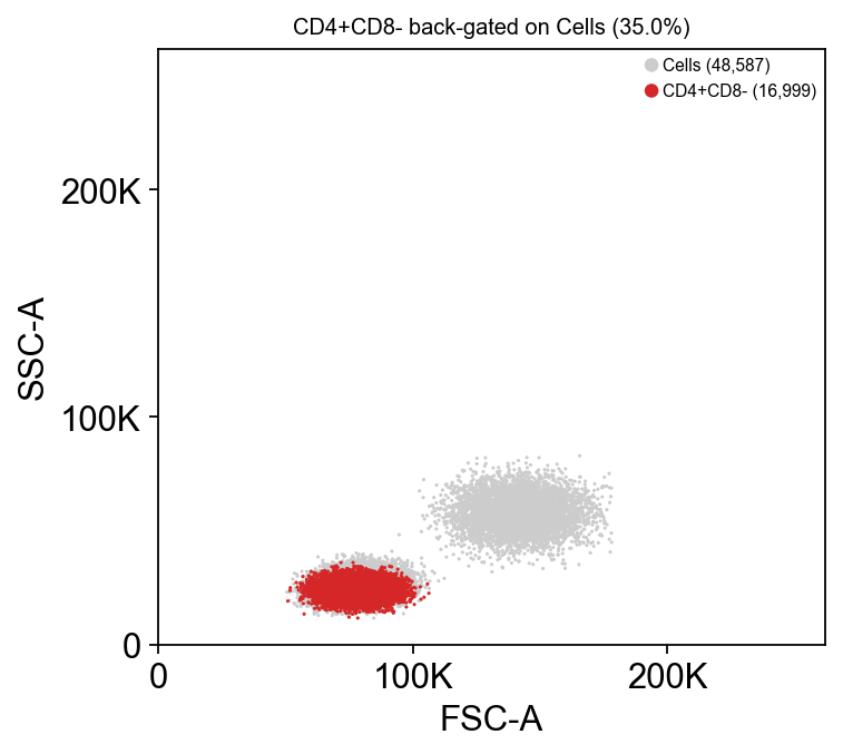
The question that catches a bad gate: where does this population sit on axes it was never gated on? A “CD4 T” population scattered through the debris corner of FSC × SSC is not a T-cell population, however clean the CD4 × CD8 plot looked — and no statistics table will tell you.
ov.flow.backgate(adata, "FSC-A", "SSC-A", result=res,
                 population="CD4+CD8-", parent="Cells",
                 transforms={"FSC-A": lin, "SSC-A": lin}, figsize=(4.8, 4.4))
None
Boolean gates#
BooleanGate composes populations that already exist, which is how “CD3+ but
not CD4+” is expressed without redrawing geometry. It is evaluated by the
strategy, since only the strategy knows what the referenced populations
resolved to.
Note that not is a separate gate: it takes exactly one operand, so “A and not
B” is two nodes rather than one. Verbose, but it means every intermediate is a
named population you can plot.
# dims=() because a boolean takes no dimensions of its own — it is evaluated
# by the strategy, the only thing that knows what its operands resolved to.
gs2 = ov.flow.GatingStrategy.from_dict(gs.to_dict())
gs2.add_gate(ov.flow.BooleanGate(name="not CD4", dims=(), operator="not",
                                 operands=("CD4+CD8-",)), parent="CD3+")
gs2.add_gate(ov.flow.BooleanGate(name="CD3+ non-CD4", dims=(), operator="and",
                                 operands=("CD3+", "not CD4")), parent="CD3+")

res2 = gs2.apply(adata.copy())
s2 = res2.stats().set_index("population")
print(f"CD3+          : {int(s2.loc['CD3+', 'count']):,}")
print(f"CD4+CD8-      : {int(s2.loc['CD4+CD8-', 'count']):,}")
print(f"CD3+ non-CD4  : {int(s2.loc['CD3+ non-CD4', 'count']):,}"
      f"   (= {int(s2.loc['CD3+', 'count']) - int(s2.loc['CD4+CD8-', 'count']):,})")
CD3+          : 28,895
CD4+CD8-      : 16,999
CD3+ non-CD4  : 11,896   (= 11,896)
What is next#
The strategy is an object, so it can be written to a file and applied to another sample — that is the next notebook.