SEACells — kernel archetypal analysis#
Persad et al. SEACells infers transcriptional and epigenomic cellular states from single-cell genomics data. Nature Biotechnology 41, 1746–1757 (2023). doi:10.1038/s41587-023-01716-9
Algorithm. Builds an adaptive Gaussian kernel on diffusion components,
then runs kernel archetypal analysis to fit n_SEACells archetypes and a
soft membership matrix A_ (cells × archetypes). Each cell is a sparse
combination of nearby archetypes.
Capabilities. soft, latent.
Strengths. Mathematically clean (explicit convex objective). Soft memberships let you do proper weighted aggregation. Native support for ATAC.
Weaknesses. O(N²) kernel construction; doesn’t scale past ~100k cells. No closed-form out-of-sample projection. GPU helps but doesn’t change the complexity.
1. Setup#
# Standard imports + omicverse defaults.
import warnings
warnings.filterwarnings('ignore')

import numpy as np
import pandas as pd
import omicverse as ov
import scvelo as scv      # only used for the demo dataset

ov.plot_set()
🔬 Starting plot initialization...
🧬 Detecting GPU devices…
✅ NVIDIA CUDA GPUs detected: 1
    • [CUDA 0] NVIDIA H100 80GB HBM3
      Memory: 79.1 GB | Compute: 9.0

   ____            _     _    __
  / __ \____ ___  (_)___| |  / /__  _____________
 / / / / __ `__ \/ / ___/ | / / _ \/ ___/ ___/ _ \
/ /_/ / / / / / / / /__ | |/ /  __/ /  (__  )  __/
\____/_/ /_/ /_/_/\___/ |___/\___/_/  /____/\___/

🔖 Version: 2.2.0   📚 Tutorials: https://omicverse.readthedocs.io/
✅ plot_set complete.
2. Load and preprocess#
# Pancreas scRNA-seq (Bastidas-Ponce et al. 2019). Standard omicverse
# preprocess flow: qc -> preprocess -> scale -> pca -> neighbors -> umap.
adata = scv.datasets.pancreas()
adata = ov.pp.qc(adata,
                 tresh={'mito_perc': 0.20, 'nUMIs': 500, 'detected_genes': 250},
                 mt_startswith='mt-')
adata = ov.pp.preprocess(adata, mode='shiftlog|pearson', n_HVGs=2000)
adata.layers['lognorm'] = adata.X.copy()        # mcRigor reads this
adata = adata[:, adata.var.highly_variable_features]
ov.pp.scale(adata)
ov.pp.pca(adata, layer='scaled', n_pcs=30)
adata.obsm['X_pca'] = adata.obsm['scaled|original|X_pca']
ov.pp.neighbors(adata, n_neighbors=15, use_rep='X_pca')
ov.pp.umap(adata)
print('adata:', adata.shape, 'celltypes:', sorted(adata.obs['clusters'].unique()))
🖥️ Using CPU mode for QC...

📊 Step 1: Calculating QC Metrics

   ✓ Gene Family Detection:
   ┌──────────────────────────────┬────────────────────┬────────────────────┐
   │ Gene Family                  │ Genes Found        │ Detection Method   │
   ├──────────────────────────────┼────────────────────┼────────────────────┤
   │ Mitochondrial                │ 13                 │ Auto (MT-)         │
   ├──────────────────────────────┼────────────────────┼────────────────────┤
   │ Ribosomal                    │ 0 ⚠️               │ Auto (RPS/RPL)     │
   ├──────────────────────────────┼────────────────────┼────────────────────┤
   │ Hemoglobin                   │ 0 ⚠️               │ Auto (regex)       │
   └──────────────────────────────┴────────────────────┴────────────────────┘

   ✓ QC Metrics Summary:
   ┌─────────────────────────┬────────────────────┬─────────────────────────┐
   │ Metric                  │ Mean               │ Range (Min - Max)       │
   ├─────────────────────────┼────────────────────┼─────────────────────────┤
   │ nUMIs                   │ 6675               │ 3020 - 18524            │
   ├─────────────────────────┼────────────────────┼─────────────────────────┤
   │ Detected Genes          │ 2516               │ 1473 - 4492             │
   ├─────────────────────────┼────────────────────┼─────────────────────────┤
   │ Mitochondrial %         │ 0.7%               │ 0.2% - 4.3%             │
   ├─────────────────────────┼────────────────────┼─────────────────────────┤
   │ Ribosomal %             │ 0.0%               │ 0.0% - 0.0%             │
   ├─────────────────────────┼────────────────────┼─────────────────────────┤
   │ Hemoglobin %            │ 0.0%               │ 0.0% - 0.0%             │
   └─────────────────────────┴────────────────────┴─────────────────────────┘

   📈 Original cell count: 3,696

🔧 Step 2: Quality Filtering (SEURAT)
   Thresholds: mito≤0.2, nUMIs≥500, genes≥250
   📊 Seurat Filter Results:
     • nUMIs filter (≥500): 0 cells failed (0.0%)
     • Genes filter (≥250): 0 cells failed (0.0%)
     • Mitochondrial filter (≤0.2): 0 cells failed (0.0%)
   ✓ Filters applied successfully
   ✓ Combined QC filters: 0 cells removed (0.0%)

🎯 Step 3: Final Filtering
   Parameters: min_genes=200, min_cells=3
   Ratios: max_genes_ratio=1, max_cells_ratio=1
✓ Final filtering: 0 cells, 12,261 genes removed

🔍 Step 4: Doublet Detection
   💡 Running pyscdblfinder (Python port of R scDblFinder)
   🔍 Running scdblfinder detection...
[ScDblFinder] wrote scDblFinder_score + scDblFinder_class — threshold=0.387
   ✓ scDblFinder completed: 66 doublets removed (1.8%)

╭─ SUMMARY: qc ──────────────────────────────────────────────────────╮
│  Duration: 19.9899s                                                │
│  Shape:    3,696 x 27,998 (Unchanged)                              │
│                                                                    │
│  CHANGES DETECTED                                                  │
│  ────────────────                                                  │
│  ● OBS    │ ✚ cell_complexity (float)                              │
│           │ ✚ detected_genes (int)                                 │
│           │ ✚ hb_perc (float)                                      │
│           │ ✚ mito_perc (float)                                    │
│           │ ✚ nUMIs (float)                                        │
│           │ ✚ n_counts (float)                                     │
│           │ ✚ n_genes (int)                                        │
│           │ ✚ n_genes_by_counts (int)                              │
│           │ ✚ passing_mt (bool)                                    │
│           │ ✚ passing_nUMIs (bool)                                 │
│           │ ✚ passing_ngenes (bool)                                │
│           │ ✚ pct_counts_hb (float)                                │
│           │ ✚ pct_counts_mt (float)                                │
│           │ ✚ pct_counts_ribo (float)                              │
│           │ ✚ ribo_perc (float)                                    │
│           │ ✚ total_counts (float)                                 │
│                                                                    │
│  ● VAR    │ ✚ hb (bool)                                            │
│           │ ✚ mt (bool)                                            │
│           │ ✚ ribo (bool)                                          │
│                                                                    │
╰────────────────────────────────────────────────────────────────────╯
🔍 [2026-05-19 18:47:25] Running preprocessing in 'cpu' mode...
Begin robust gene identification
    After filtration, 15737/15737 genes are kept.
    Among 15737 genes, 15736 genes are robust.
✅ Robust gene identification completed successfully.
Begin size normalization: shiftlog and HVGs selection pearson
🔍 Count Normalization:
   Target sum: 500000.0
   Exclude highly expressed: True
   Max fraction threshold: 0.2
   ⚠️ Excluding 1 highly-expressed genes from normalization computation
   Excluded genes: ['Ghrl']
✅ Count Normalization Completed Successfully!
   ✓ Processed: 3,630 cells × 15,736 genes
   ✓ Runtime: 0.24s

🔍 Highly Variable Genes Selection (Experimental):
   Method: pearson_residuals
   Target genes: 2,000
   Theta (overdispersion): 100
✅ Experimental HVG Selection Completed Successfully!
   ✓ Selected: 2,000 highly variable genes out of 15,736 total (12.7%)
   ✓ Results added to AnnData object:
     • 'highly_variable': Boolean vector (adata.var)
     • 'highly_variable_rank': Float vector (adata.var)
     • 'highly_variable_nbatches': Int vector (adata.var)
     • 'highly_variable_intersection': Boolean vector (adata.var)
     • 'means': Float vector (adata.var)
     • 'variances': Float vector (adata.var)
     • 'residual_variances': Float vector (adata.var)
    Time to analyze data in cpu: 1.41 seconds.
✅ Preprocessing completed successfully.
    Added:
        'highly_variable_features', boolean vector (adata.var)
        'means', float vector (adata.var)
        'variances', float vector (adata.var)
        'residual_variances', float vector (adata.var)
        'counts', raw counts layer (adata.layers)
    End of size normalization: shiftlog and HVGs selection pearson

╭─ SUMMARY: preprocess ──────────────────────────────────────────────╮
│  Duration: 1.7944s                                                 │
│  Shape:    3,630 x 15,737 -> 3,630 x 15,736                        │
│                                                                    │
│  CHANGES DETECTED                                                  │
│  ────────────────                                                  │
│  ● VAR    │ ✚ highly_variable (bool)                               │
│           │ ✚ highly_variable_features (bool)                      │
│           │ ✚ highly_variable_rank (float)                         │
│           │ ✚ means (float)                                        │
│           │ ✚ n_cells (int)                                        │
│           │ ✚ percent_cells (float)                                │
│           │ ✚ residual_variances (float)                           │
│           │ ✚ robust (bool)                                        │
│           │ ✚ variances (float)                                    │
│                                                                    │
│  ● UNS    │ ✚ history_log                                          │
│           │ ✚ hvg                                                  │
│           │ ✚ log1p                                                │
│                                                                    │
│  ● LAYERS │ ✚ counts (sparse matrix, 3630x15736)                   │
│                                                                    │
╰────────────────────────────────────────────────────────────────────╯
╭─ SUMMARY: scale ───────────────────────────────────────────────────╮
│  Duration: 0.6413s                                                 │
│  Shape:    3,630 x 2,000 (Unchanged)                               │
│                                                                    │
│  CHANGES DETECTED                                                  │
│  ────────────────                                                  │
│  ● LAYERS │ ✚ scaled (array, 3630x2000)                            │
│                                                                    │
╰────────────────────────────────────────────────────────────────────╯
computing PCA🔍
    with n_comps=30
   🖥️ Using sklearn PCA for CPU computation
   🖥️ sklearn PCA backend: CPU computation
   📊 PCA input data type: ArrayView, shape: (3630, 2000), dtype: float64
🔧 PCA solver used: covariance_eigh
    finished✅ (1.33s)

╭─ SUMMARY: pca ─────────────────────────────────────────────────────╮
│  Duration: 1.335s                                                  │
│  Shape:    3,630 x 2,000 (Unchanged)                               │
│                                                                    │
│  CHANGES DETECTED                                                  │
│  ────────────────                                                  │
│  ● UNS    │ ✚ scaled|original|cum_sum_eigenvalues                  │
│           │ ✚ scaled|original|pca_var_ratios                       │
│                                                                    │
│  ● OBSM   │ ✚ scaled|original|X_pca (array, 3630x30)               │
│                                                                    │
╰────────────────────────────────────────────────────────────────────╯
🖥️ Using Scanpy CPU to calculate neighbors...

🔍 K-Nearest Neighbors Graph Construction:
   Mode: cpu
   Neighbors: 15
   Method: umap
   Metric: euclidean
   Representation: X_pca
   🔍 Computing neighbor distances...
🔍 Computing connectivity matrix...
   💡 Using UMAP-style connectivity
✓ Graph is fully connected

✅ KNN Graph Construction Completed Successfully!
   ✓ Processed: 3,630 cells with 15 neighbors each
   ✓ Results added to AnnData object:
     • 'neighbors': Neighbors metadata (adata.uns)
     • 'distances': Distance matrix (adata.obsp)
     • 'connectivities': Connectivity matrix (adata.obsp)

╭─ SUMMARY: neighbors ───────────────────────────────────────────────╮
│  Duration: 8.4831s                                                 │
│  Shape:    3,630 x 2,000 (Unchanged)                               │
│                                                                    │
│  CHANGES DETECTED                                                  │
│  ────────────────                                                  │
╰────────────────────────────────────────────────────────────────────╯
🔍 [2026-05-19 18:47:37] Running UMAP in 'cpu' mode...
🖥️ Using Scanpy CPU UMAP...

🔍 UMAP Dimensionality Reduction:
   Mode: cpu
   Method: umap
   Components: 2
   Min distance: 0.5
{'n_neighbors': 15, 'method': 'umap', 'random_state': 0, 'metric': 'euclidean', 'use_rep': 'X_pca'}
   🔍 Computing UMAP parameters...
   🔍 Computing UMAP embedding (classic method)...
✅ UMAP Dimensionality Reduction Completed Successfully!
   ✓ Embedding shape: 3,630 cells × 2 dimensions
   ✓ Results added to AnnData object:
     • 'X_umap': UMAP coordinates (adata.obsm)
     • 'umap': UMAP parameters (adata.uns)
✅ UMAP completed successfully.

╭─ SUMMARY: umap ────────────────────────────────────────────────────╮
│  Duration: 1.2196s                                                 │
│  Shape:    3,630 x 2,000 (Unchanged)                               │
│                                                                    │
│  CHANGES DETECTED                                                  │
│  ────────────────                                                  │
│  ● UNS    │ ✚ umap                                                 │
│           │ └─ params: {'a': 0.5830300199950147, 'b': 1.334166993228519}│
│                                                                    │
╰────────────────────────────────────────────────────────────────────╯
adata: (3630, 2000) celltypes: ['Alpha', 'Beta', 'Delta', 'Ductal', 'Epsilon', 'Ngn3 high EP', 'Ngn3 low EP', 'Pre-endocrine']
3. Fit SEACells#
Build the kernel on X_pca and fit 100 archetypes. device='cuda' would
move Franke–Wolfe onto the GPU (requires cupy); the default CPU path is
plenty fast on this 3.6 k-cell dataset.
mc = ov.single.MetaCell(
    adata.copy(), method='seacells', n_metacells=100,
    use_rep='X_pca', device='cpu', random_state=0,
).fit()
print(f'fit done: {mc.method}, runtime={mc._fit_result.runtime_s:.2f} s')
Welcome to SEACells!
Parameter graph_construction = union being used to build KNN graph...
Building kernel on X_pca
fit done: seacells, runtime=17.46 s
4. AnnData schema after fit#
Every backend writes the same fields into adata — that’s what lets the
downstream helpers below work without branching on the backend.
# Inspect what the fit wrote into adata via the unified schema.
print(f'method      : {mc.method}')
print(f'capabilities: {sorted(mc.capabilities)}')
print(f'n_metacells : {np.unique(mc._fit_result.assignments).size}')
print(f'runtime     : {mc._fit_result.runtime_s:.3f} s')
print(f'uns         : {dict(mc.adata.uns["metacell"])}')
method      : seacells
capabilities: ['latent', 'soft']
n_metacells : 100
runtime     : 17.461 s
uns         : {'method': 'seacells', 'n_metacells': 100, 'n_iter': 11, 'converged': True, 'runtime_s': 17.460611820220947, 'random_state': 0, 'capabilities': ['latent', 'soft']}
5. Aggregate to a metacell AnnData#
predicted(method='hard', layer='counts', summary='sum') returns a
metacell × gene AnnData with raw count totals preserved — the format that
downstream tools (SCENIC, CellPhoneDB, pseudobulk DE) actually want.
ad_mc = mc.predicted(method='hard', layer='counts', summary='sum',
                     celltype_label='clusters')
print(f'metacell AnnData: {ad_mc.shape}')
print(f'mean cells/metacell: {ad_mc.obs["n_cells"].mean():.1f}')
ad_mc.obs.head()
metacell AnnData: (100, 2000)
mean cells/metacell: 36.3
| n_cells | clusters | clusters_purity | |
|---|---|---|---|
| mc-0 | 26 | Ngn3 high EP | 0.692308 |
| mc-1 | 14 | Epsilon | 1.000000 |
| mc-2 | 44 | Ngn3 high EP | 1.000000 |
| mc-3 | 61 | Alpha | 0.967213 |
| mc-4 | 23 | Ductal | 1.000000 |
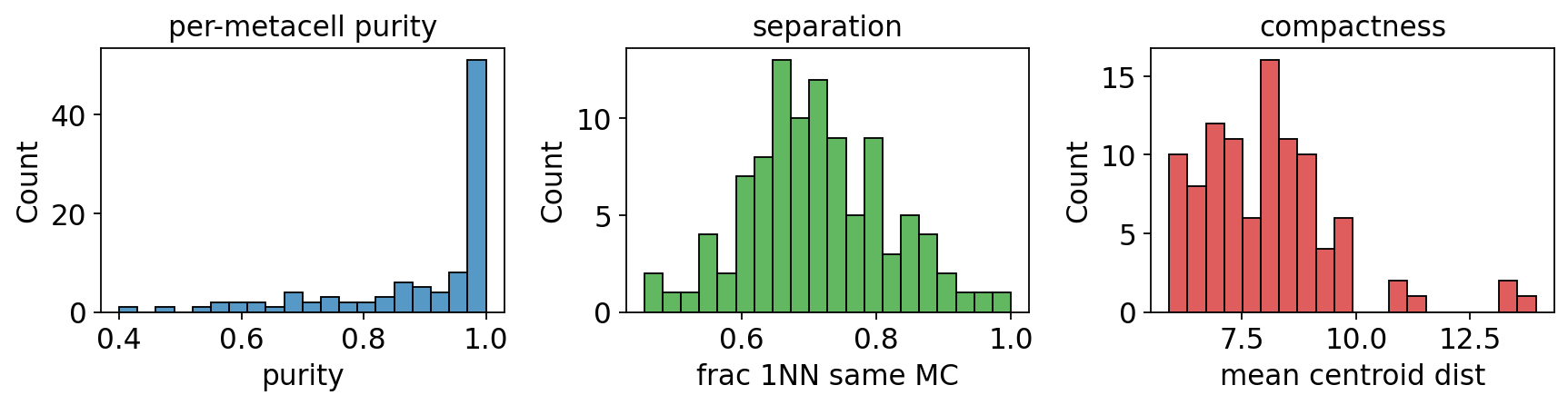
6. Benchmarking metrics (purity / separation / compactness)#
# Compute purity / separation / compactness AND show the 3-panel histogram
# in one call (ov.pl.metacell_metrics returns the per-metacell tables too).
purity, separation, compactness = ov.pl.metacell_metrics(
    mc, label_key='clusters', use_rep='X_pca',
)
7. mcRigor: statistical validation#
For each metacell, mcRigor permutes the (cells × genes) submatrix in two
ways and asks: is the observed gene–gene covariance bigger than the null
distribution at this metacell’s size? Metacells whose mcDiv exceeds the
size-stratified threshold are flagged as 'dubious'.
# mcRigor's double-permutation null. dubious_rate = fraction of cells in
# heterogeneous metacells; rigor_score = 1 - 0.5*(dubious_rate + zero_rate).
rep = mc.check_rigor(layer_lognorm='lognorm', n_rep=20,
                     feature_use=1000, random_state=0)
print(f'rigor_score : {rep.score:.3f}')
print(f'dubious_rate: {rep.dubious_rate:.3f}')
print(f'zero_rate   : {rep.zero_rate:.3f}')
print(f'# metacells : {rep.n_metacells}')
rigor_score : 0.640
dubious_rate: 0.477
zero_rate   : 0.243
# metacells : 100
7.1 Per-metacell mcDiv vs size#
# mcDiv vs metacell size, overlaid with size-stratified threshold.
ov.pl.rigor_scatter(rep)
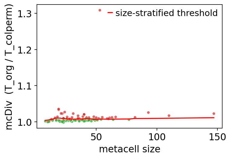
<Axes: xlabel='metacell size', ylabel='mcDiv (T_org / T_colperm)'>
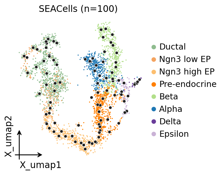
8. UMAP with metacell centroids#
# UMAP coloured by celltype with metacell centroids overlaid in dark grey.
import matplotlib.pyplot as plt
fig, ax = plt.subplots(figsize=(5, 4))
ov.pl.embedding(mc.adata, basis='X_umap', color='clusters', ax=ax, show=False,
                frameon='small', title='SEACells (n=100)', size=12)
labels = mc._fit_result.assignments
pts = np.array([mc.adata.obsm['X_umap'][labels == u].mean(axis=0)
                for u in np.unique(labels)])
ax.scatter(pts[:, 0], pts[:, 1], s=24, c='#222',
           edgecolors='white', linewidths=0.6, zorder=5)
plt.tight_layout(); plt.show()
9. Per-celltype purity boxplot#
# Per-celltype boxplot of metacell purity.
ov.pl.metacell_purity_box(mc, label_key='clusters')
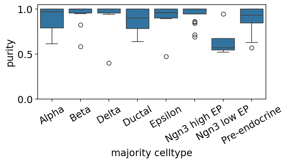
<Axes: xlabel='majority celltype', ylabel='purity'>
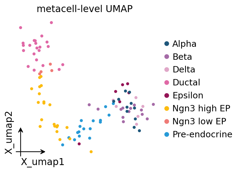
10. Metacell-level UMAP#
A common downstream use of metacells is to treat them as a much smaller “atlas” of pseudo-cells and re-run the standard omicverse preprocess → PCA → UMAP loop on them. Cell-type signal should survive.
# Treat the metacell AnnData as a smaller dataset and run the standard
# omicverse preprocess -> pca -> neighbors -> umap loop on it.
ad_mc = ov.pp.preprocess(ad_mc, mode='shiftlog|pearson',
                          n_HVGs=min(2000, ad_mc.n_vars))
ad_mc = ad_mc[:, ad_mc.var.highly_variable_features]
ov.pp.scale(ad_mc)
ov.pp.pca(ad_mc, layer='scaled', n_pcs=min(30, ad_mc.n_obs - 1))
ad_mc.obsm['X_pca'] = ad_mc.obsm['scaled|original|X_pca']
ov.pp.neighbors(ad_mc, n_neighbors=min(15, ad_mc.n_obs - 1), use_rep='X_pca')
ov.pp.umap(ad_mc)
ov.pl.embedding(ad_mc, basis='X_umap', color='clusters',
                frameon='small', title='metacell-level UMAP', size=80)
🔍 [2026-05-19 18:48:19] Running preprocessing in 'cpu' mode...
Begin robust gene identification
    After filtration, 2000/2000 genes are kept.
    Among 2000 genes, 2000 genes are robust.
✅ Robust gene identification completed successfully.
Begin size normalization: shiftlog and HVGs selection pearson

🔍 Count Normalization:
   Target sum: 500000.0
   Exclude highly expressed: True
   Max fraction threshold: 0.2
   ⚠️ Excluding 1 highly-expressed genes from normalization computation
   Excluded genes: ['Ghrl']

✅ Count Normalization Completed Successfully!
   ✓ Processed: 100 cells × 2,000 genes
   ✓ Runtime: 0.00s

🔍 Highly Variable Genes Selection (Experimental):
   Method: pearson_residuals
   Target genes: 2,000
   Theta (overdispersion): 100

✅ Experimental HVG Selection Completed Successfully!
   ✓ Selected: 2,000 highly variable genes out of 2,000 total (100.0%)
   ✓ Results added to AnnData object:
     • 'highly_variable': Boolean vector (adata.var)
     • 'highly_variable_rank': Float vector (adata.var)
     • 'highly_variable_nbatches': Int vector (adata.var)
     • 'highly_variable_intersection': Boolean vector (adata.var)
     • 'means': Float vector (adata.var)
     • 'variances': Float vector (adata.var)
     • 'residual_variances': Float vector (adata.var)
    Time to analyze data in cpu: 0.03 seconds.
✅ Preprocessing completed successfully.
    Added:
        'highly_variable_features', boolean vector (adata.var)
        'means', float vector (adata.var)
        'variances', float vector (adata.var)
        'residual_variances', float vector (adata.var)
        'counts', raw counts layer (adata.layers)
    End of size normalization: shiftlog and HVGs selection pearson

╭─ SUMMARY: preprocess ──────────────────────────────────────────────╮
│  Duration: 0.0446s                                                 │
│  Shape:    100 x 2,000 (Unchanged)                                 │
│                                                                    │
│  CHANGES DETECTED                                                  │
│  ────────────────                                                  │
│  ● UNS    │ ✚ REFERENCE_MANU                                       │
│           │ ✚ _ov_provenance                                       │
│           │ ✚ history_log                                          │
│           │ ✚ hvg                                                  │
│           │ ✚ log1p                                                │
│           │ ✚ status                                               │
│           │ ✚ status_args                                          │
│                                                                    │
│  ● LAYERS │ ✚ counts (sparse matrix, 100x2000)                     │
│                                                                    │
╰────────────────────────────────────────────────────────────────────╯

╭─ SUMMARY: scale ───────────────────────────────────────────────────╮
│  Duration: 0.014s                                                  │
│  Shape:    100 x 2,000 (Unchanged)                                 │
│                                                                    │
│  CHANGES DETECTED                                                  │
│  ────────────────                                                  │
│  ● LAYERS │ ✚ scaled (array, 100x2000)                             │
│                                                                    │
╰────────────────────────────────────────────────────────────────────╯
computing PCA🔍
    with n_comps=30
   🖥️ Using sklearn PCA for CPU computation
   🖥️ sklearn PCA backend: CPU computation
   📊 PCA input data type: ArrayView, shape: (100, 2000), dtype: float64
🔧 PCA solver used: covariance_eigh
    finished✅ (1.39s)

╭─ SUMMARY: pca ─────────────────────────────────────────────────────╮
│  Duration: 1.3952s                                                 │
│  Shape:    100 x 2,000 (Unchanged)                                 │
│                                                                    │
│  CHANGES DETECTED                                                  │
│  ────────────────                                                  │
│  ● UNS    │ ✚ pca                                                  │
│           │ └─ params: {'zero_center': True, 'use_highly_variable': Tr...│
│           │ ✚ scaled|original|cum_sum_eigenvalues                  │
│           │ ✚ scaled|original|pca_var_ratios                       │
│                                                                    │
│  ● OBSM   │ ✚ X_pca (array, 100x30)                                │
│           │ ✚ scaled|original|X_pca (array, 100x30)                │
│                                                                    │
╰────────────────────────────────────────────────────────────────────╯
🖥️ Using Scanpy CPU to calculate neighbors...

🔍 K-Nearest Neighbors Graph Construction:
   Mode: cpu
   Neighbors: 15
   Method: umap
   Metric: euclidean
   Representation: X_pca
   🔍 Computing neighbor distances...
   🔍 Computing connectivity matrix...
   💡 Using UMAP-style connectivity
   ✓ Graph is fully connected

✅ KNN Graph Construction Completed Successfully!
   ✓ Processed: 100 cells with 15 neighbors each
   ✓ Results added to AnnData object:
     • 'neighbors': Neighbors metadata (adata.uns)
     • 'distances': Distance matrix (adata.obsp)
     • 'connectivities': Connectivity matrix (adata.obsp)

╭─ SUMMARY: neighbors ───────────────────────────────────────────────╮
│  Duration: 0.1199s                                                 │
│  Shape:    100 x 2,000 (Unchanged)                                 │
│                                                                    │
│  CHANGES DETECTED                                                  │
│  ────────────────                                                  │
│  ● UNS    │ ✚ neighbors                                            │
│           │ └─ params: {'n_neighbors': 15, 'method': 'umap', 'random_s...│
│                                                                    │
│  ● OBSP   │ ✚ connectivities (sparse matrix, 100x100)              │
│           │ ✚ distances (sparse matrix, 100x100)                   │
│                                                                    │
╰────────────────────────────────────────────────────────────────────╯
🔍 [2026-05-19 18:48:21] Running UMAP in 'cpu' mode...
🖥️ Using Scanpy CPU UMAP...

🔍 UMAP Dimensionality Reduction:
   Mode: cpu
   Method: umap
   Components: 2
   Min distance: 0.5
{'n_neighbors': 15, 'method': 'umap', 'random_state': 0, 'metric': 'euclidean', 'use_rep': 'X_pca'}
   🔍 Computing UMAP parameters...
   🔍 Computing UMAP embedding (classic method)...

✅ UMAP Dimensionality Reduction Completed Successfully!
   ✓ Embedding shape: 100 cells × 2 dimensions
   ✓ Results added to AnnData object:
     • 'X_umap': UMAP coordinates (adata.obsm)
     • 'umap': UMAP parameters (adata.uns)
✅ UMAP completed successfully.

╭─ SUMMARY: umap ────────────────────────────────────────────────────╮
│  Duration: 0.0112s                                                 │
│  Shape:    100 x 2,000 (Unchanged)                                 │
│                                                                    │
│  CHANGES DETECTED                                                  │
│  ────────────────                                                  │
│  ● UNS    │ ✚ umap                                                 │
│           │ └─ params: {'a': 0.5830300199950147, 'b': 1.334166993228519}│
│                                                                    │
│  ● OBSM   │ ✚ X_umap (array, 100x2)                                │
│                                                                    │
╰────────────────────────────────────────────────────────────────────╯
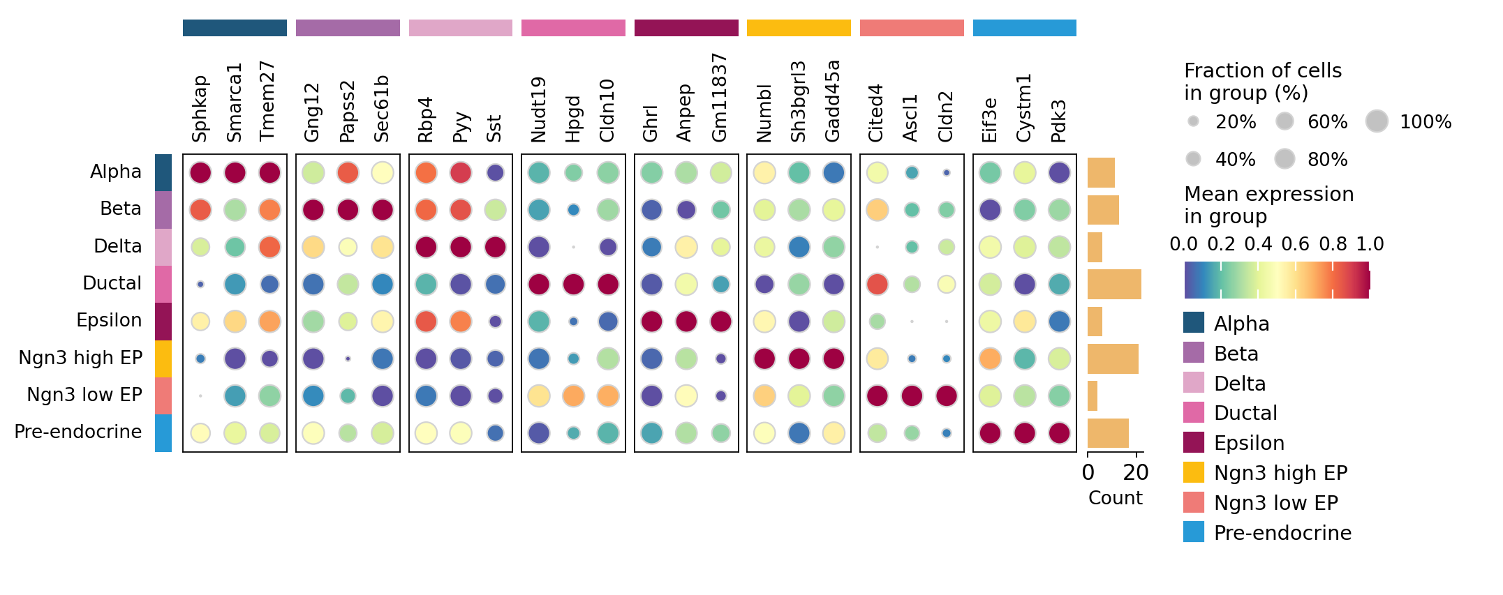
11. Top markers per celltype on the metacell AnnData#
# Find top markers per celltype on the metacell AnnData (omicverse helper —
# drops the categories with <2 metacells automatically and reports cell-type
# fractions ``pts`` along with the gene names).
counts = ad_mc.obs['clusters'].value_counts()
keep = counts[counts >= 2].index.tolist()
ad_mc_for_de = ad_mc[ad_mc.obs['clusters'].isin(keep)].copy()
ad_mc_for_de.obs['clusters'] = ad_mc_for_de.obs['clusters'].astype('category')

ov.single.find_markers(ad_mc_for_de, groupby='clusters', method='wilcoxon',
                       key_added='rank_genes_groups', pts=True, use_gpu=False)
ov.single.get_markers(ad_mc_for_de, n_genes=3, key='rank_genes_groups')
🔍 Finding marker genes | method: wilcoxon | groupby: clusters | n_groups: 8 | n_genes: 50
✅ Done | 8 groups × 50 genes | corr: benjamini-hochberg | stored in adata.uns['rank_genes_groups']
| group | rank | names | scores | logfoldchanges | pvals | pvals_adj | pct_group | pct_rest | |
|---|---|---|---|---|---|---|---|---|---|
| 0 | Alpha | 1 | Sphkap | 5.381498 | 5.620847 | 7.386865e-08 | 2.077214e-05 | 1.0 | 0.449438 |
| 1 | Alpha | 2 | Smarca1 | 5.348449 | 3.378446 | 8.871137e-08 | 2.077214e-05 | 1.0 | 0.988764 |
| 2 | Alpha | 3 | Tmem27 | 5.337432 | 6.293408 | 9.427214e-08 | 2.077214e-05 | 1.0 | 0.808989 |
| 3 | Beta | 1 | Gng12 | 5.796038 | 4.034294 | 6.789978e-09 | 2.672994e-06 | 1.0 | 1.000000 |
| 4 | Beta | 2 | Papss2 | 5.785789 | 5.529241 | 7.217283e-09 | 2.672994e-06 | 1.0 | 0.609195 |
| 5 | Beta | 3 | Sec61b | 5.765290 | 1.695018 | 8.151753e-09 | 2.672994e-06 | 1.0 | 1.000000 |
| 6 | Delta | 1 | Rbp4 | 4.092979 | 5.551823 | 4.258667e-05 | 9.540831e-03 | 1.0 | 1.000000 |
| 7 | Delta | 2 | Pyy | 4.092979 | 5.879094 | 4.258667e-05 | 9.540831e-03 | 1.0 | 1.000000 |
| 8 | Delta | 3 | Sst | 4.078465 | 11.871149 | 4.533409e-05 | 9.540831e-03 | 1.0 | 0.691489 |
| 9 | Ductal | 1 | Nudt19 | 7.139349 | 3.294932 | 9.377431e-13 | 8.161789e-11 | 1.0 | 1.000000 |
| 10 | Ductal | 2 | Hpgd | 7.139349 | 6.828624 | 9.377431e-13 | 8.161789e-11 | 1.0 | 0.358974 |
| 11 | Ductal | 3 | Cldn10 | 7.131028 | 3.775280 | 9.962235e-13 | 8.161789e-11 | 1.0 | 0.961538 |
| 12 | Epsilon | 1 | Ghrl | 4.092979 | 10.756620 | 4.258667e-05 | 6.525540e-03 | 1.0 | 0.978723 |
| 13 | Epsilon | 2 | Anpep | 4.092979 | 4.274902 | 4.258667e-05 | 6.525540e-03 | 1.0 | 0.946809 |
| 14 | Epsilon | 3 | Gm11837 | 4.078465 | 6.213355 | 4.533409e-05 | 6.525540e-03 | 1.0 | 0.585106 |
| 15 | Ngn3 high EP | 1 | Numbl | 6.968998 | 3.258245 | 3.192060e-12 | 1.419333e-09 | 1.0 | 0.898734 |
| 16 | Ngn3 high EP | 2 | Sh3bgrl3 | 6.918222 | 1.446357 | 4.573467e-12 | 1.419333e-09 | 1.0 | 1.000000 |
| 17 | Ngn3 high EP | 3 | Gadd45a | 6.909760 | 4.950183 | 4.854760e-12 | 1.419333e-09 | 1.0 | 0.987342 |
| 18 | Ngn3 low EP | 1 | Cited4 | 3.377268 | 3.317390 | 7.320963e-04 | 1.229936e-01 | 1.0 | 0.833333 |
| 19 | Ngn3 low EP | 2 | Ascl1 | 3.377268 | 5.349068 | 7.320963e-04 | 1.229936e-01 | 1.0 | 0.364583 |
| 20 | Ngn3 low EP | 3 | Cldn2 | 3.342088 | 5.082502 | 8.315059e-04 | 1.229936e-01 | 1.0 | 0.322917 |
| 21 | Pre-endocrine | 1 | Eif3e | 6.216927 | 0.865488 | 5.069873e-10 | 5.697706e-07 | 1.0 | 1.000000 |
| 22 | Pre-endocrine | 2 | Cystm1 | 6.198574 | 1.286395 | 5.697706e-10 | 5.697706e-07 | 1.0 | 1.000000 |
| 23 | Pre-endocrine | 3 | Pdk3 | 6.024225 | 2.548138 | 1.699222e-09 | 7.012711e-07 | 1.0 | 1.000000 |
# Dotplot of top markers per metacell-level celltype.
ov.pl.markers_dotplot(ad_mc_for_de, groupby='clusters', n_genes=3,
                      key='rank_genes_groups')
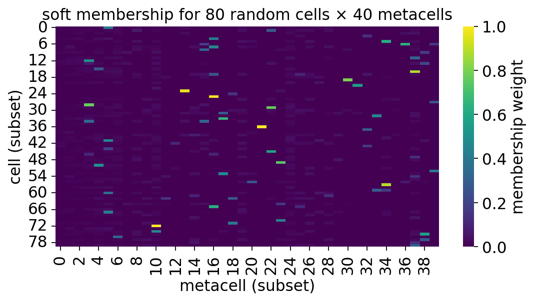
12. SEACells-specific: soft membership matrix#
A_ is the per-cell sparse soft-membership over archetypes — what makes
SEACells different from a hard partitioner. Most cells are explained by
1–3 archetypes; the rest of the row is exactly zero. This is what enables
weighted aggregation in DE / velocity / cell–cell communication.
# Heatmap of soft membership for a random subset of cells × metacells.
ov.pl.metacell_soft_heatmap(mc, n_cells=80, n_mc=40, random_state=0)
<Axes: title={'center': 'soft membership for 80 random cells × 40 metacells'}, xlabel='metacell (subset)', ylabel='cell (subset)'>
# Quick stats on how many archetypes each cell touches.
soft = mc.soft_membership().tocsr()
nnz_per_cell = (soft > 0).sum(axis=1).A1
print(f'soft membership shape   : {soft.shape}')
print(f'mean archetypes per cell: {nnz_per_cell.mean():.2f}')
print(f'sparsity                : {1 - soft.nnz / (soft.shape[0]*soft.shape[1]):.4f}')
pd.Series(nnz_per_cell).value_counts().sort_index().head(8)
soft membership shape   : (3630, 100)
mean archetypes per cell: 13.22
sparsity                : 0.8678
1    269
2    343
3    230
4    163
5    129
6     97
7    101
8     82
Name: count, dtype: int64
13. Save / load roundtrip#
# Save/load roundtrip — every backend supports this.
import tempfile, os
with tempfile.NamedTemporaryFile(suffix='.pkl', delete=False) as f:
    path = f.name
mc.save(path)

mc2 = ov.single.MetaCell(adata.copy(), method='seacells', n_metacells=100,
                          use_rep='X_pca', random_state=0)
mc2.load(path)
print(f'saved+loaded {path}')
os.remove(path)
saved+loaded /tmp/tmprzkhlmzr.pkl
14. Takeaways#
SEACells gives you a soft membership every other backend (except MetaQ via top-k cosine) lacks. This is what makes weighted-aggregate DE and RNA-velocity-on-metacells work.
O(N²) kernel construction is the bottleneck — on this 3.6 k-cell dataset it’s fine on CPU; past 100 k cells the
cupyGPU mode is essential and past 1 M cells switch tometaqormc2.For atlas workflows requiring out-of-sample projection, use
metaqinstead.