Recommended workflow: SEACells end-to-end + downstream sanity#
This is the default tutorial for users new to ov.single.MetaCell. We
run the recommended backend ('seacells') on a typical single-sample
dataset and immediately drive it into the two most common downstream
analyses — differential expression and marker-dotplot — to show that the
metacell-level AnnData is a drop-in replacement for the cell-level one.
After this notebook:
Run
t_metacell_multisampleif you have ≥2 samples / batches.Browse zoo/index if you want to swap out the backend (faster:
kmeans/supercell; out-of-sample:metaq; sanity floor:random).
1. Setup#
import warnings
warnings.filterwarnings('ignore')

import numpy as np
import pandas as pd
import omicverse as ov
import scvelo as scv   # demo dataset only

ov.plot_set()
🔬 Starting plot initialization...
🧬 Detecting GPU devices…
✅ NVIDIA CUDA GPUs detected: 1
    • [CUDA 0] NVIDIA H100 80GB HBM3
      Memory: 79.1 GB | Compute: 9.0

   ____            _     _    __
  / __ \____ ___  (_)___| |  / /__  _____________
 / / / / __ `__ \/ / ___/ | / / _ \/ ___/ ___/ _ \
/ /_/ / / / / / / / /__ | |/ /  __/ /  (__  )  __/
\____/_/ /_/ /_/_/\___/ |___/\___/_/  /____/\___/

🔖 Version: 2.2.0   📚 Tutorials: https://omicverse.readthedocs.io/
✅ plot_set complete.
2. Load and preprocess#
Standard omicverse flow: qc → preprocess → scale → pca → neighbors → umap.
SEACells builds its kernel on a low-dim embedding (here X_pca).
adata = scv.datasets.pancreas()
adata = ov.pp.qc(adata,
                 tresh={'mito_perc': 0.20, 'nUMIs': 500, 'detected_genes': 250},
                 mt_startswith='mt-')
adata = ov.pp.preprocess(adata, mode='shiftlog|pearson', n_HVGs=2000)
adata.layers['lognorm'] = adata.X.copy()
adata = adata[:, adata.var.highly_variable_features]
ov.pp.scale(adata)
ov.pp.pca(adata, layer='scaled', n_pcs=30)
adata.obsm['X_pca'] = adata.obsm['scaled|original|X_pca']
ov.pp.neighbors(adata, n_neighbors=15, use_rep='X_pca')
ov.pp.umap(adata)
print('adata:', adata.shape, 'celltypes:', sorted(adata.obs['clusters'].unique()))
🖥️ Using CPU mode for QC...

📊 Step 1: Calculating QC Metrics

   ✓ Gene Family Detection:
   ┌──────────────────────────────┬────────────────────┬────────────────────┐
   │ Gene Family                  │ Genes Found        │ Detection Method   │
   ├──────────────────────────────┼────────────────────┼────────────────────┤
   │ Mitochondrial                │ 13                 │ Auto (MT-)         │
   ├──────────────────────────────┼────────────────────┼────────────────────┤
   │ Ribosomal                    │ 0 ⚠️               │ Auto (RPS/RPL)     │
   ├──────────────────────────────┼────────────────────┼────────────────────┤
   │ Hemoglobin                   │ 0 ⚠️               │ Auto (regex)       │
   └──────────────────────────────┴────────────────────┴────────────────────┘

   ✓ QC Metrics Summary:
   ┌─────────────────────────┬────────────────────┬─────────────────────────┐
   │ Metric                  │ Mean               │ Range (Min - Max)       │
   ├─────────────────────────┼────────────────────┼─────────────────────────┤
   │ nUMIs                   │ 6675               │ 3020 - 18524            │
   ├─────────────────────────┼────────────────────┼─────────────────────────┤
   │ Detected Genes          │ 2516               │ 1473 - 4492             │
   ├─────────────────────────┼────────────────────┼─────────────────────────┤
   │ Mitochondrial %         │ 0.7%               │ 0.2% - 4.3%             │
   ├─────────────────────────┼────────────────────┼─────────────────────────┤
   │ Ribosomal %             │ 0.0%               │ 0.0% - 0.0%             │
   ├─────────────────────────┼────────────────────┼─────────────────────────┤
   │ Hemoglobin %            │ 0.0%               │ 0.0% - 0.0%             │
   └─────────────────────────┴────────────────────┴─────────────────────────┘

   📈 Original cell count: 3,696

🔧 Step 2: Quality Filtering (SEURAT)
   Thresholds: mito≤0.2, nUMIs≥500, genes≥250
   📊 Seurat Filter Results:
     • nUMIs filter (≥500): 0 cells failed (0.0%)
     • Genes filter (≥250): 0 cells failed (0.0%)
     • Mitochondrial filter (≤0.2): 0 cells failed (0.0%)
   ✓ Filters applied successfully
   ✓ Combined QC filters: 0 cells removed (0.0%)

🎯 Step 3: Final Filtering
   Parameters: min_genes=200, min_cells=3
   Ratios: max_genes_ratio=1, max_cells_ratio=1
✓ Final filtering: 0 cells, 12,261 genes removed

🔍 Step 4: Doublet Detection
   💡 Running pyscdblfinder (Python port of R scDblFinder)
   🔍 Running scdblfinder detection...
[ScDblFinder] wrote scDblFinder_score + scDblFinder_class — threshold=0.387
   ✓ scDblFinder completed: 66 doublets removed (1.8%)

╭─ SUMMARY: qc ──────────────────────────────────────────────────────╮
│  Duration: 18.8586s                                                │
│  Shape:    3,696 x 27,998 (Unchanged)                              │
│                                                                    │
│  CHANGES DETECTED                                                  │
│  ────────────────                                                  │
│  ● OBS    │ ✚ cell_complexity (float)                              │
│           │ ✚ detected_genes (int)                                 │
│           │ ✚ hb_perc (float)                                      │
│           │ ✚ mito_perc (float)                                    │
│           │ ✚ nUMIs (float)                                        │
│           │ ✚ n_counts (float)                                     │
│           │ ✚ n_genes (int)                                        │
│           │ ✚ n_genes_by_counts (int)                              │
│           │ ✚ passing_mt (bool)                                    │
│           │ ✚ passing_nUMIs (bool)                                 │
│           │ ✚ passing_ngenes (bool)                                │
│           │ ✚ pct_counts_hb (float)                                │
│           │ ✚ pct_counts_mt (float)                                │
│           │ ✚ pct_counts_ribo (float)                              │
│           │ ✚ ribo_perc (float)                                    │
│           │ ✚ total_counts (float)                                 │
│                                                                    │
│  ● VAR    │ ✚ hb (bool)                                            │
│           │ ✚ mt (bool)                                            │
│           │ ✚ ribo (bool)                                          │
│                                                                    │
╰────────────────────────────────────────────────────────────────────╯
🔍 [2026-05-19 18:44:27] Running preprocessing in 'cpu' mode...
Begin robust gene identification
    After filtration, 15737/15737 genes are kept.
    Among 15737 genes, 15736 genes are robust.
✅ Robust gene identification completed successfully.
Begin size normalization: shiftlog and HVGs selection pearson
🔍 Count Normalization:
   Target sum: 500000.0
   Exclude highly expressed: True
   Max fraction threshold: 0.2
   ⚠️ Excluding 1 highly-expressed genes from normalization computation
   Excluded genes: ['Ghrl']
✅ Count Normalization Completed Successfully!
   ✓ Processed: 3,630 cells × 15,736 genes
   ✓ Runtime: 0.24s

🔍 Highly Variable Genes Selection (Experimental):
   Method: pearson_residuals
   Target genes: 2,000
   Theta (overdispersion): 100
✅ Experimental HVG Selection Completed Successfully!
   ✓ Selected: 2,000 highly variable genes out of 15,736 total (12.7%)
   ✓ Results added to AnnData object:
     • 'highly_variable': Boolean vector (adata.var)
     • 'highly_variable_rank': Float vector (adata.var)
     • 'highly_variable_nbatches': Int vector (adata.var)
     • 'highly_variable_intersection': Boolean vector (adata.var)
     • 'means': Float vector (adata.var)
     • 'variances': Float vector (adata.var)
     • 'residual_variances': Float vector (adata.var)
    Time to analyze data in cpu: 1.48 seconds.
✅ Preprocessing completed successfully.
    Added:
        'highly_variable_features', boolean vector (adata.var)
        'means', float vector (adata.var)
        'variances', float vector (adata.var)
        'residual_variances', float vector (adata.var)
        'counts', raw counts layer (adata.layers)
    End of size normalization: shiftlog and HVGs selection pearson

╭─ SUMMARY: preprocess ──────────────────────────────────────────────╮
│  Duration: 1.8644s                                                 │
│  Shape:    3,630 x 15,737 -> 3,630 x 15,736                        │
│                                                                    │
│  CHANGES DETECTED                                                  │
│  ────────────────                                                  │
│  ● VAR    │ ✚ highly_variable (bool)                               │
│           │ ✚ highly_variable_features (bool)                      │
│           │ ✚ highly_variable_rank (float)                         │
│           │ ✚ means (float)                                        │
│           │ ✚ n_cells (int)                                        │
│           │ ✚ percent_cells (float)                                │
│           │ ✚ residual_variances (float)                           │
│           │ ✚ robust (bool)                                        │
│           │ ✚ variances (float)                                    │
│                                                                    │
│  ● UNS    │ ✚ history_log                                          │
│           │ ✚ hvg                                                  │
│           │ ✚ log1p                                                │
│                                                                    │
│  ● LAYERS │ ✚ counts (sparse matrix, 3630x15736)                   │
│                                                                    │
╰────────────────────────────────────────────────────────────────────╯
╭─ SUMMARY: scale ───────────────────────────────────────────────────╮
│  Duration: 0.6108s                                                 │
│  Shape:    3,630 x 2,000 (Unchanged)                               │
│                                                                    │
│  CHANGES DETECTED                                                  │
│  ────────────────                                                  │
│  ● LAYERS │ ✚ scaled (array, 3630x2000)                            │
│                                                                    │
╰────────────────────────────────────────────────────────────────────╯
computing PCA🔍
    with n_comps=30
   🖥️ Using sklearn PCA for CPU computation
   🖥️ sklearn PCA backend: CPU computation
   📊 PCA input data type: ArrayView, shape: (3630, 2000), dtype: float64
🔧 PCA solver used: covariance_eigh
    finished✅ (2.21s)

╭─ SUMMARY: pca ─────────────────────────────────────────────────────╮
│  Duration: 2.2184s                                                 │
│  Shape:    3,630 x 2,000 (Unchanged)                               │
│                                                                    │
│  CHANGES DETECTED                                                  │
│  ────────────────                                                  │
│  ● UNS    │ ✚ scaled|original|cum_sum_eigenvalues                  │
│           │ ✚ scaled|original|pca_var_ratios                       │
│                                                                    │
│  ● OBSM   │ ✚ scaled|original|X_pca (array, 3630x30)               │
│                                                                    │
╰────────────────────────────────────────────────────────────────────╯
🖥️ Using Scanpy CPU to calculate neighbors...

🔍 K-Nearest Neighbors Graph Construction:
   Mode: cpu
   Neighbors: 15
   Method: umap
   Metric: euclidean
   Representation: X_pca
   🔍 Computing neighbor distances...
🔍 Computing connectivity matrix...
   💡 Using UMAP-style connectivity
✓ Graph is fully connected

✅ KNN Graph Construction Completed Successfully!
   ✓ Processed: 3,630 cells with 15 neighbors each
   ✓ Results added to AnnData object:
     • 'neighbors': Neighbors metadata (adata.uns)
     • 'distances': Distance matrix (adata.obsp)
     • 'connectivities': Connectivity matrix (adata.obsp)

╭─ SUMMARY: neighbors ───────────────────────────────────────────────╮
│  Duration: 8.4673s                                                 │
│  Shape:    3,630 x 2,000 (Unchanged)                               │
│                                                                    │
│  CHANGES DETECTED                                                  │
│  ────────────────                                                  │
╰────────────────────────────────────────────────────────────────────╯
🔍 [2026-05-19 18:44:41] Running UMAP in 'cpu' mode...
🖥️ Using Scanpy CPU UMAP...

🔍 UMAP Dimensionality Reduction:
   Mode: cpu
   Method: umap
   Components: 2
   Min distance: 0.5
{'n_neighbors': 15, 'method': 'umap', 'random_state': 0, 'metric': 'euclidean', 'use_rep': 'X_pca'}
   🔍 Computing UMAP parameters...
   🔍 Computing UMAP embedding (classic method)...
✅ UMAP Dimensionality Reduction Completed Successfully!
   ✓ Embedding shape: 3,630 cells × 2 dimensions
   ✓ Results added to AnnData object:
     • 'X_umap': UMAP coordinates (adata.obsm)
     • 'umap': UMAP parameters (adata.uns)
✅ UMAP completed successfully.

╭─ SUMMARY: umap ────────────────────────────────────────────────────╮
│  Duration: 0.8242s                                                 │
│  Shape:    3,630 x 2,000 (Unchanged)                               │
│                                                                    │
│  CHANGES DETECTED                                                  │
│  ────────────────                                                  │
│  ● UNS    │ ✚ umap                                                 │
│           │ └─ params: {'a': 0.5830300199950147, 'b': 1.334166993228519}│
│                                                                    │
╰────────────────────────────────────────────────────────────────────╯
adata: (3630, 2000) celltypes: ['Alpha', 'Beta', 'Delta', 'Ductal', 'Epsilon', 'Ngn3 high EP', 'Ngn3 low EP', 'Pre-endocrine']
3. Fit SEACells#
n_metacells = adata.n_obs // 50 is a reasonable starting point — it gives
~70–80 metacells per 4 k cells, with mean metacell size ~50 cells.
mc = ov.single.MetaCell(
    adata.copy(), method='seacells',
    n_metacells=adata.n_obs // 50,
    use_rep='X_pca', device='cpu', random_state=0,
).fit()
print(f'fit done: n_metacells={mc.n_metacells}, '
      f'runtime={mc._fit_result.runtime_s:.2f} s, '
      f'capabilities={sorted(mc.capabilities)}')
Welcome to SEACells!
Parameter graph_construction = union being used to build KNN graph...
Building kernel on X_pca
fit done: n_metacells=72, runtime=11.64 s, capabilities=['latent', 'soft']
4. Aggregate to a metacell AnnData#
# 'sum' aggregation preserves raw-count totals — required by SCENIC / pseudobulk
# DE / CellPhoneDB. Use 'mean' for visualization-only workflows.
ad_mc = mc.predicted(method='soft', layer='counts', summary='sum',
                     celltype_label='clusters')
print(f'metacell AnnData: {ad_mc.shape}')
print(f'  mean cells/metacell: {ad_mc.obs["n_cells"].mean():.1f}')
print(f'  mean purity        : {ad_mc.obs["clusters_purity"].mean():.3f}')
ad_mc.obs.head()
metacell AnnData: (72, 2000)
  mean cells/metacell: 111.4
  mean purity        : 0.877
| n_cells | clusters | clusters_purity | |
|---|---|---|---|
| mc-0 | 200 | Alpha | 0.979167 |
| mc-1 | 45 | Epsilon | 1.000000 |
| mc-2 | 152 | Beta | 1.000000 |
| mc-3 | 112 | Beta | 1.000000 |
| mc-4 | 92 | Ductal | 0.975000 |
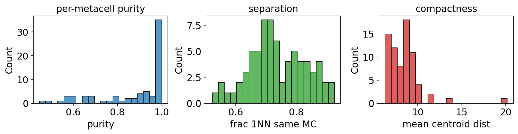
5. Quality check: purity / separation / compactness#
These three SEACells-style metrics apply to any metacell partition. All three are computed in one helper call and the histograms tell you whether the partition is honest.
purity, separation, compactness = ov.pl.metacell_metrics(
    mc, label_key='clusters', use_rep='X_pca',
)
6. mcRigor: statistical validation#
Asks per metacell: is its gene–gene covariance larger than expected from a
within-cell gene-shuffle null at this metacell size? Metacells whose
mcDiv exceeds the size-stratified threshold are flagged as 'dubious'.
Lower dubious_rate → tighter metacells.
rep = mc.check_rigor(layer_lognorm='lognorm', n_rep=30,
                     feature_use=1000, random_state=0)
print(f'rigor_score : {rep.score:.3f}')
print(f'dubious_rate: {rep.dubious_rate:.3f}')
print(f'zero_rate   : {rep.zero_rate:.3f}')
rigor_score : 0.555
dubious_rate: 0.647
zero_rate   : 0.243
ov.pl.rigor_scatter(rep)
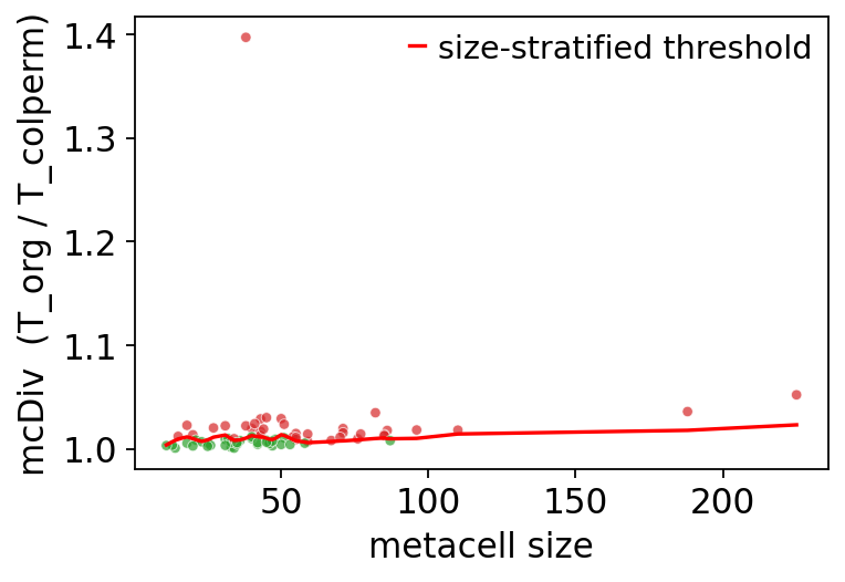
<Axes: xlabel='metacell size', ylabel='mcDiv (T_org / T_colperm)'>
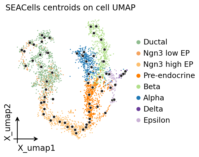
7. Visualize: metacell centroids on the source UMAP#
Centroids inside clearly-coloured cell-type islands = good metacells. Centroids straddling cell-type boundaries → mixed metacells (high mcDiv, low purity).
import matplotlib.pyplot as plt
fig, ax = plt.subplots(figsize=(5, 4))
ov.pl.embedding(mc.adata, basis='X_umap', color='clusters', ax=ax, show=False,
                frameon='small', title='SEACells centroids on cell UMAP', size=12)
labels = mc._fit_result.assignments
pts = np.array([mc.adata.obsm['X_umap'][labels == u].mean(axis=0)
                for u in np.unique(labels)])
ax.scatter(pts[:, 0], pts[:, 1], s=24, c='#222',
           edgecolors='white', linewidths=0.6, zorder=5)
plt.tight_layout(); plt.show()
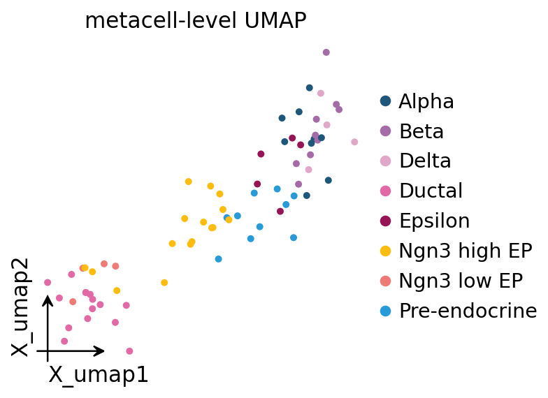
8. Visualize: metacell-level UMAP#
A common downstream use of metacells is to treat them as a much smaller atlas — re-run the standard preprocess → PCA → UMAP loop on the aggregated AnnData. Celltype structure should survive cleanly.
ad_mc = ov.pp.preprocess(ad_mc, mode='shiftlog|pearson',
                          n_HVGs=min(2000, ad_mc.n_vars))
ad_mc = ad_mc[:, ad_mc.var.highly_variable_features]
ov.pp.scale(ad_mc)
ov.pp.pca(ad_mc, layer='scaled', n_pcs=min(30, ad_mc.n_obs - 1))
ad_mc.obsm['X_pca'] = ad_mc.obsm['scaled|original|X_pca']
ov.pp.neighbors(ad_mc, n_neighbors=min(15, ad_mc.n_obs - 1), use_rep='X_pca')
ov.pp.umap(ad_mc)
ov.pl.embedding(ad_mc, basis='X_umap', color='clusters',
                frameon='small', title='metacell-level UMAP', size=80)
🔍 [2026-05-19 18:45:28] Running preprocessing in 'cpu' mode...
Begin robust gene identification
    After filtration, 2000/2000 genes are kept.
    Among 2000 genes, 2000 genes are robust.
✅ Robust gene identification completed successfully.
Begin size normalization: shiftlog and HVGs selection pearson

🔍 Count Normalization:
   Target sum: 500000.0
   Exclude highly expressed: True
   Max fraction threshold: 0.2
   ⚠️ Excluding 1 highly-expressed genes from normalization computation
   Excluded genes: ['Ghrl']

✅ Count Normalization Completed Successfully!
   ✓ Processed: 72 cells × 2,000 genes
   ✓ Runtime: 0.00s

🔍 Highly Variable Genes Selection (Experimental):
   Method: pearson_residuals
   Target genes: 2,000
   Theta (overdispersion): 100

✅ Experimental HVG Selection Completed Successfully!
   ✓ Selected: 2,000 highly variable genes out of 2,000 total (100.0%)
   ✓ Results added to AnnData object:
     • 'highly_variable': Boolean vector (adata.var)
     • 'highly_variable_rank': Float vector (adata.var)
     • 'highly_variable_nbatches': Int vector (adata.var)
     • 'highly_variable_intersection': Boolean vector (adata.var)
     • 'means': Float vector (adata.var)
     • 'variances': Float vector (adata.var)
     • 'residual_variances': Float vector (adata.var)
    Time to analyze data in cpu: 0.03 seconds.
✅ Preprocessing completed successfully.
    Added:
        'highly_variable_features', boolean vector (adata.var)
        'means', float vector (adata.var)
        'variances', float vector (adata.var)
        'residual_variances', float vector (adata.var)
        'counts', raw counts layer (adata.layers)
    End of size normalization: shiftlog and HVGs selection pearson

╭─ SUMMARY: preprocess ──────────────────────────────────────────────╮
│  Duration: 0.0383s                                                 │
│  Shape:    72 x 2,000 (Unchanged)                                  │
│                                                                    │
│  CHANGES DETECTED                                                  │
│  ────────────────                                                  │
│  ● UNS    │ ✚ REFERENCE_MANU                                       │
│           │ ✚ _ov_provenance                                       │
│           │ ✚ history_log                                          │
│           │ ✚ hvg                                                  │
│           │ ✚ log1p                                                │
│           │ ✚ status                                               │
│           │ ✚ status_args                                          │
│                                                                    │
│  ● LAYERS │ ✚ counts (sparse matrix, 72x2000)                      │
│                                                                    │
╰────────────────────────────────────────────────────────────────────╯

╭─ SUMMARY: scale ───────────────────────────────────────────────────╮
│  Duration: 0.0131s                                                 │
│  Shape:    72 x 2,000 (Unchanged)                                  │
│                                                                    │
│  CHANGES DETECTED                                                  │
│  ────────────────                                                  │
│  ● LAYERS │ ✚ scaled (array, 72x2000)                              │
│                                                                    │
╰────────────────────────────────────────────────────────────────────╯
computing PCA🔍
    with n_comps=30
   🖥️ Using sklearn PCA for CPU computation
   🖥️ sklearn PCA backend: CPU computation
   📊 PCA input data type: ArrayView, shape: (72, 2000), dtype: float64
🔧 PCA solver used: covariance_eigh
    finished✅ (0.92s)

╭─ SUMMARY: pca ─────────────────────────────────────────────────────╮
│  Duration: 0.9311s                                                 │
│  Shape:    72 x 2,000 (Unchanged)                                  │
│                                                                    │
│  CHANGES DETECTED                                                  │
│  ────────────────                                                  │
│  ● UNS    │ ✚ pca                                                  │
│           │ └─ params: {'zero_center': True, 'use_highly_variable': Tr...│
│           │ ✚ scaled|original|cum_sum_eigenvalues                  │
│           │ ✚ scaled|original|pca_var_ratios                       │
│                                                                    │
│  ● OBSM   │ ✚ X_pca (array, 72x30)                                 │
│           │ ✚ scaled|original|X_pca (array, 72x30)                 │
│                                                                    │
╰────────────────────────────────────────────────────────────────────╯
🖥️ Using Scanpy CPU to calculate neighbors...

🔍 K-Nearest Neighbors Graph Construction:
   Mode: cpu
   Neighbors: 15
   Method: umap
   Metric: euclidean
   Representation: X_pca
   🔍 Computing neighbor distances...
   🔍 Computing connectivity matrix...
   💡 Using UMAP-style connectivity
   ✓ Graph is fully connected

✅ KNN Graph Construction Completed Successfully!
   ✓ Processed: 72 cells with 15 neighbors each
   ✓ Results added to AnnData object:
     • 'neighbors': Neighbors metadata (adata.uns)
     • 'distances': Distance matrix (adata.obsp)
     • 'connectivities': Connectivity matrix (adata.obsp)

╭─ SUMMARY: neighbors ───────────────────────────────────────────────╮
│  Duration: 0.138s                                                  │
│  Shape:    72 x 2,000 (Unchanged)                                  │
│                                                                    │
│  CHANGES DETECTED                                                  │
│  ────────────────                                                  │
│  ● UNS    │ ✚ neighbors                                            │
│           │ └─ params: {'n_neighbors': 15, 'method': 'umap', 'random_s...│
│                                                                    │
│  ● OBSP   │ ✚ connectivities (sparse matrix, 72x72)                │
│           │ ✚ distances (sparse matrix, 72x72)                     │
│                                                                    │
╰────────────────────────────────────────────────────────────────────╯
🔍 [2026-05-19 18:45:29] Running UMAP in 'cpu' mode...
🖥️ Using Scanpy CPU UMAP...

🔍 UMAP Dimensionality Reduction:
   Mode: cpu
   Method: umap
   Components: 2
   Min distance: 0.5
{'n_neighbors': 15, 'method': 'umap', 'random_state': 0, 'metric': 'euclidean', 'use_rep': 'X_pca'}
   🔍 Computing UMAP parameters...
   🔍 Computing UMAP embedding (classic method)...

✅ UMAP Dimensionality Reduction Completed Successfully!
   ✓ Embedding shape: 72 cells × 2 dimensions
   ✓ Results added to AnnData object:
     • 'X_umap': UMAP coordinates (adata.obsm)
     • 'umap': UMAP parameters (adata.uns)
✅ UMAP completed successfully.

╭─ SUMMARY: umap ────────────────────────────────────────────────────╮
│  Duration: 0.0097s                                                 │
│  Shape:    72 x 2,000 (Unchanged)                                  │
│                                                                    │
│  CHANGES DETECTED                                                  │
│  ────────────────                                                  │
│  ● UNS    │ ✚ umap                                                 │
│           │ └─ params: {'a': 0.5830300199950147, 'b': 1.334166993228519}│
│                                                                    │
│  ● OBSM   │ ✚ X_umap (array, 72x2)                                 │
│                                                                    │
╰────────────────────────────────────────────────────────────────────╯
9. Downstream task 1 — differential expression#
Find marker genes per celltype on the metacell AnnData using
ov.single.find_markers (the omicverse Wilcoxon wrapper with pts=True
for per-cluster expression fractions).
# Drop celltypes with <2 metacells (find_markers needs n>=2 per group).
counts = ad_mc.obs['clusters'].value_counts()
keep = counts[counts >= 2].index.tolist()
ad_mc_de = ad_mc[ad_mc.obs['clusters'].isin(keep)].copy()
ad_mc_de.obs['clusters'] = ad_mc_de.obs['clusters'].astype('category')

ov.single.find_markers(ad_mc_de, groupby='clusters', method='wilcoxon',
                       key_added='rank_genes_groups', pts=True, use_gpu=False)
ov.single.get_markers(ad_mc_de, n_genes=3, key='rank_genes_groups')
🔍 Finding marker genes | method: wilcoxon | groupby: clusters | n_groups: 8 | n_genes: 50
✅ Done | 8 groups × 50 genes | corr: benjamini-hochberg | stored in adata.uns['rank_genes_groups']
| group | rank | names | scores | logfoldchanges | pvals | pvals_adj | pct_group | pct_rest | |
|---|---|---|---|---|---|---|---|---|---|
| 0 | Alpha | 1 | Asb4 | 4.827149 | 5.818245 | 1.385013e-06 | 2.418402e-04 | 1.0 | 0.523810 |
| 1 | Alpha | 2 | Smarca1 | 4.776068 | 3.182478 | 1.787557e-06 | 2.418402e-04 | 1.0 | 1.000000 |
| 2 | Alpha | 3 | Ocrl | 4.776068 | 3.136611 | 1.787557e-06 | 2.418402e-04 | 1.0 | 0.984127 |
| 3 | Beta | 1 | Gng12 | 4.827149 | 3.927392 | 1.385013e-06 | 1.934722e-04 | 1.0 | 1.000000 |
| 4 | Beta | 2 | Sec61b | 4.827149 | 1.642527 | 1.385013e-06 | 1.934722e-04 | 1.0 | 1.000000 |
| 5 | Beta | 3 | Gm27033 | 4.827149 | 3.917109 | 1.385013e-06 | 1.934722e-04 | 1.0 | 0.952381 |
| 6 | Delta | 1 | Cd24a | 3.343364 | 2.544938 | 8.276928e-04 | 4.196597e-02 | 1.0 | 1.000000 |
| 7 | Delta | 2 | Spock3 | 3.343364 | 5.352329 | 8.276928e-04 | 4.196597e-02 | 1.0 | 0.750000 |
| 8 | Delta | 3 | Mest | 3.343364 | 4.213267 | 8.276928e-04 | 4.196597e-02 | 1.0 | 1.000000 |
| 9 | Ductal | 1 | Tkt | 5.927646 | 1.698946 | 3.073082e-09 | 1.241199e-07 | 1.0 | 1.000000 |
| 10 | Ductal | 2 | Proser2 | 5.927646 | 2.839478 | 3.073082e-09 | 1.241199e-07 | 1.0 | 0.982456 |
| 11 | Ductal | 3 | Nudt19 | 5.927646 | 3.226622 | 3.073082e-09 | 1.241199e-07 | 1.0 | 1.000000 |
| 12 | Epsilon | 1 | Txndc12 | 3.710407 | 1.429926 | 2.069260e-04 | 1.620964e-02 | 1.0 | 1.000000 |
| 13 | Epsilon | 2 | Foxd3 | 3.710407 | 8.726132 | 2.069260e-04 | 1.620964e-02 | 1.0 | 0.044776 |
| 14 | Epsilon | 3 | Gm11837 | 3.710407 | 5.789987 | 2.069260e-04 | 1.620964e-02 | 1.0 | 0.895522 |
| 15 | Ngn3 high EP | 1 | Cbfa2t3 | 6.054562 | 3.596581 | 1.408005e-09 | 2.708256e-07 | 1.0 | 0.946429 |
| 16 | Ngn3 high EP | 2 | Sh3bgrl3 | 6.054562 | 1.468390 | 1.408005e-09 | 2.708256e-07 | 1.0 | 1.000000 |
| 17 | Ngn3 high EP | 3 | Rnf114 | 6.041017 | 1.807264 | 1.531460e-09 | 2.708256e-07 | 1.0 | 1.000000 |
| 18 | Ngn3 low EP | 1 | Cited4 | 3.343364 | 2.892943 | 8.276928e-04 | 8.960757e-02 | 1.0 | 0.941176 |
| 19 | Ngn3 low EP | 2 | Cldn2 | 3.294197 | 4.624810 | 9.870337e-04 | 8.960757e-02 | 1.0 | 0.588235 |
| 20 | Ngn3 low EP | 3 | Ascl1 | 3.269613 | 4.734896 | 1.076946e-03 | 8.960757e-02 | 1.0 | 0.588235 |
| 21 | Pre-endocrine | 1 | Eif3e | 5.015152 | 0.868462 | 5.299167e-07 | 1.744158e-04 | 1.0 | 1.000000 |
| 22 | Pre-endocrine | 2 | Cystm1 | 4.966303 | 1.284075 | 6.824141e-07 | 1.744158e-04 | 1.0 | 1.000000 |
| 23 | Pre-endocrine | 3 | Foxp1 | 4.950020 | 1.440488 | 7.420595e-07 | 1.744158e-04 | 1.0 | 1.000000 |
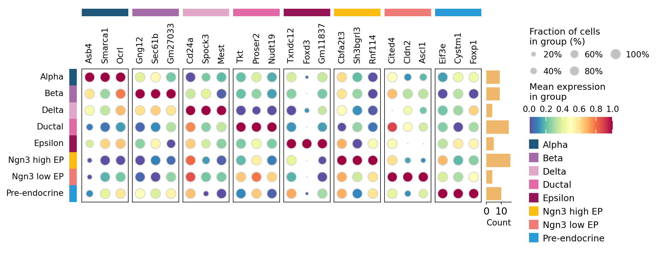
10. Downstream task 2 — marker dotplot#
ov.pl.markers_dotplot reads the rank_genes_groups result and shows the
top-N markers per group with both expression intensity (colour) and the
fraction of metacells in which each gene is expressed (dot size).
Canonical pancreas markers (Ins1/Ins2 for Beta, Gcg for Alpha, etc.)
should pop out clearly even on this small metacell set.
ov.pl.markers_dotplot(ad_mc_de, groupby='clusters', n_genes=3,
                      key='rank_genes_groups')
11. Save the metacell partition#
Save the slim state (assignments + soft membership + config). The
companion load recovers the unified AnnData schema and lets you re-run
predicted() / compute_purity() / etc. without re-fitting.
import tempfile, os
with tempfile.NamedTemporaryFile(suffix='.pkl', delete=False) as f:
    path = f.name
mc.save(path)
print(f'saved to {path}')
os.remove(path)
saved to /tmp/tmpet9z7zry.pkl
12. Next steps#
Multi-sample data? Move on to t_metacell_multisample — same workflow but with batch correction first so per-sample metacells live in a shared embedding.
Need out-of-sample assignment (new cells arrive over time)? Switch the backend to
metaqand usemc.assign_new_cells(adata_new)— see zoo/t_metacell_metaq.Want to validate the choice of backend? Run
ov.single.compare_metacell_backendson your data — see zoo/t_metacell_compare.Want to use metacells in cell–cell communication / SCENIC? Pass
ad_mc(the AnnData returned bymc.predicted()) into the standardov.single.pCellPhoneDB,ov.single.pySCENIC, etc. workflows — they consume the unified schema directly.