random — the honest lower-bound baseline#
Algorithm. Uniformly assign each cell to one of n_metacells buckets.
No use of any feature or graph information. Optional stratify_key
restricts the random assignment to within each stratum.
Capabilities. None. This is intentional — random is the floor
that every other metacell method must beat to justify its complexity.
Why is this in the zoo? Recent benchmarks have argued that random
subsampling may be close to “principled” metacells for many downstream
tasks. Running random on your own data is the single best way to
falsify or confirm this for your pipeline.
Choosing the stratification key matters. Stratifying by a column that already encodes celltype structure (Leiden at the resolution most notebooks use, or — obviously — the celltype label itself) leaks the evaluation signal back into the baseline. Section 12 shows this explicitly. The honest baseline here is uniform random — that’s what every other backend must beat.
1. Setup#
# Standard imports + omicverse defaults.
import warnings
warnings.filterwarnings('ignore')

import numpy as np
import pandas as pd
import omicverse as ov
import scvelo as scv      # only used for the demo dataset

ov.plot_set()
🔬 Starting plot initialization...
🧬 Detecting GPU devices…
✅ NVIDIA CUDA GPUs detected: 1
    • [CUDA 0] NVIDIA H100 80GB HBM3
      Memory: 79.1 GB | Compute: 9.0

   ____            _     _    __
  / __ \____ ___  (_)___| |  / /__  _____________
 / / / / __ `__ \/ / ___/ | / / _ \/ ___/ ___/ _ \
/ /_/ / / / / / / / /__ | |/ /  __/ /  (__  )  __/
\____/_/ /_/ /_/_/\___/ |___/\___/_/  /____/\___/

🔖 Version: 2.2.0   📚 Tutorials: https://omicverse.readthedocs.io/
✅ plot_set complete.
2. Load and preprocess#
Standard omicverse flow. We also compute a Leiden clustering — not for the primary baseline below, but for the section-12 diagnostic showing why Leiden-stratified random is misleading on this dataset.
# Pancreas scRNA-seq + Leiden clustering. Leiden is used as the stratification
# key below — it's the *honest* baseline (knows only the coarse graph community,
# not the celltype label we evaluate against).
adata = scv.datasets.pancreas()
adata = ov.pp.qc(adata,
                 tresh={'mito_perc': 0.20, 'nUMIs': 500, 'detected_genes': 250},
                 mt_startswith='mt-')
adata = ov.pp.preprocess(adata, mode='shiftlog|pearson', n_HVGs=2000)
adata.layers['lognorm'] = adata.X.copy()
adata = adata[:, adata.var.highly_variable_features]
ov.pp.scale(adata)
ov.pp.pca(adata, layer='scaled', n_pcs=30)
adata.obsm['X_pca'] = adata.obsm['scaled|original|X_pca']
ov.pp.neighbors(adata, n_neighbors=15, use_rep='X_pca')
ov.pp.umap(adata)
ov.pp.leiden(adata, resolution=0.8)
print('adata:', adata.shape,
      '\n celltypes (eval) :', sorted(adata.obs['clusters'].unique()),
      '\n leiden clusters  :', adata.obs['leiden'].nunique())
🖥️ Using CPU mode for QC...

📊 Step 1: Calculating QC Metrics

   ✓ Gene Family Detection:
   ┌──────────────────────────────┬────────────────────┬────────────────────┐
   │ Gene Family                  │ Genes Found        │ Detection Method   │
   ├──────────────────────────────┼────────────────────┼────────────────────┤
   │ Mitochondrial                │ 13                 │ Auto (MT-)         │
   ├──────────────────────────────┼────────────────────┼────────────────────┤
   │ Ribosomal                    │ 0 ⚠️               │ Auto (RPS/RPL)     │
   ├──────────────────────────────┼────────────────────┼────────────────────┤
   │ Hemoglobin                   │ 0 ⚠️               │ Auto (regex)       │
   └──────────────────────────────┴────────────────────┴────────────────────┘

   ✓ QC Metrics Summary:
   ┌─────────────────────────┬────────────────────┬─────────────────────────┐
   │ Metric                  │ Mean               │ Range (Min - Max)       │
   ├─────────────────────────┼────────────────────┼─────────────────────────┤
   │ nUMIs                   │ 6675               │ 3020 - 18524            │
   ├─────────────────────────┼────────────────────┼─────────────────────────┤
   │ Detected Genes          │ 2516               │ 1473 - 4492             │
   ├─────────────────────────┼────────────────────┼─────────────────────────┤
   │ Mitochondrial %         │ 0.7%               │ 0.2% - 4.3%             │
   ├─────────────────────────┼────────────────────┼─────────────────────────┤
   │ Ribosomal %             │ 0.0%               │ 0.0% - 0.0%             │
   ├─────────────────────────┼────────────────────┼─────────────────────────┤
   │ Hemoglobin %            │ 0.0%               │ 0.0% - 0.0%             │
   └─────────────────────────┴────────────────────┴─────────────────────────┘

   📈 Original cell count: 3,696

🔧 Step 2: Quality Filtering (SEURAT)
   Thresholds: mito≤0.2, nUMIs≥500, genes≥250
   📊 Seurat Filter Results:
     • nUMIs filter (≥500): 0 cells failed (0.0%)
     • Genes filter (≥250): 0 cells failed (0.0%)
     • Mitochondrial filter (≤0.2): 0 cells failed (0.0%)
   ✓ Filters applied successfully
   ✓ Combined QC filters: 0 cells removed (0.0%)

🎯 Step 3: Final Filtering
   Parameters: min_genes=200, min_cells=3
   Ratios: max_genes_ratio=1, max_cells_ratio=1
✓ Final filtering: 0 cells, 12,261 genes removed

🔍 Step 4: Doublet Detection
   💡 Running pyscdblfinder (Python port of R scDblFinder)
   🔍 Running scdblfinder detection...
[ScDblFinder] wrote scDblFinder_score + scDblFinder_class — threshold=0.387
   ✓ scDblFinder completed: 66 doublets removed (1.8%)

╭─ SUMMARY: qc ──────────────────────────────────────────────────────╮
│  Duration: 16.254s                                                 │
│  Shape:    3,696 x 27,998 (Unchanged)                              │
│                                                                    │
│  CHANGES DETECTED                                                  │
│  ────────────────                                                  │
│  ● OBS    │ ✚ cell_complexity (float)                              │
│           │ ✚ detected_genes (int)                                 │
│           │ ✚ hb_perc (float)                                      │
│           │ ✚ mito_perc (float)                                    │
│           │ ✚ nUMIs (float)                                        │
│           │ ✚ n_counts (float)                                     │
│           │ ✚ n_genes (int)                                        │
│           │ ✚ n_genes_by_counts (int)                              │
│           │ ✚ passing_mt (bool)                                    │
│           │ ✚ passing_nUMIs (bool)                                 │
│           │ ✚ passing_ngenes (bool)                                │
│           │ ✚ pct_counts_hb (float)                                │
│           │ ✚ pct_counts_mt (float)                                │
│           │ ✚ pct_counts_ribo (float)                              │
│           │ ✚ ribo_perc (float)                                    │
│           │ ✚ total_counts (float)                                 │
│                                                                    │
│  ● VAR    │ ✚ hb (bool)                                            │
│           │ ✚ mt (bool)                                            │
│           │ ✚ ribo (bool)                                          │
│                                                                    │
╰────────────────────────────────────────────────────────────────────╯
🔍 [2026-05-19 18:05:25] Running preprocessing in 'cpu' mode...
Begin robust gene identification
    After filtration, 15737/15737 genes are kept.
    Among 15737 genes, 15736 genes are robust.
✅ Robust gene identification completed successfully.
Begin size normalization: shiftlog and HVGs selection pearson
🔍 Count Normalization:
   Target sum: 500000.0
   Exclude highly expressed: True
   Max fraction threshold: 0.2
   ⚠️ Excluding 1 highly-expressed genes from normalization computation
   Excluded genes: ['Ghrl']
✅ Count Normalization Completed Successfully!
   ✓ Processed: 3,630 cells × 15,736 genes
   ✓ Runtime: 0.27s

🔍 Highly Variable Genes Selection (Experimental):
   Method: pearson_residuals
   Target genes: 2,000
   Theta (overdispersion): 100
✅ Experimental HVG Selection Completed Successfully!
   ✓ Selected: 2,000 highly variable genes out of 15,736 total (12.7%)
   ✓ Results added to AnnData object:
     • 'highly_variable': Boolean vector (adata.var)
     • 'highly_variable_rank': Float vector (adata.var)
     • 'highly_variable_nbatches': Int vector (adata.var)
     • 'highly_variable_intersection': Boolean vector (adata.var)
     • 'means': Float vector (adata.var)
     • 'variances': Float vector (adata.var)
     • 'residual_variances': Float vector (adata.var)
    Time to analyze data in cpu: 1.57 seconds.
✅ Preprocessing completed successfully.
    Added:
        'highly_variable_features', boolean vector (adata.var)
        'means', float vector (adata.var)
        'variances', float vector (adata.var)
        'residual_variances', float vector (adata.var)
        'counts', raw counts layer (adata.layers)
    End of size normalization: shiftlog and HVGs selection pearson

╭─ SUMMARY: preprocess ──────────────────────────────────────────────╮
│  Duration: 1.9519s                                                 │
│  Shape:    3,630 x 15,737 -> 3,630 x 15,736                        │
│                                                                    │
│  CHANGES DETECTED                                                  │
│  ────────────────                                                  │
│  ● VAR    │ ✚ highly_variable (bool)                               │
│           │ ✚ highly_variable_features (bool)                      │
│           │ ✚ highly_variable_rank (float)                         │
│           │ ✚ means (float)                                        │
│           │ ✚ n_cells (int)                                        │
│           │ ✚ percent_cells (float)                                │
│           │ ✚ residual_variances (float)                           │
│           │ ✚ robust (bool)                                        │
│           │ ✚ variances (float)                                    │
│                                                                    │
│  ● UNS    │ ✚ history_log                                          │
│           │ ✚ hvg                                                  │
│           │ ✚ log1p                                                │
│                                                                    │
│  ● LAYERS │ ✚ counts (sparse matrix, 3630x15736)                   │
│                                                                    │
╰────────────────────────────────────────────────────────────────────╯
╭─ SUMMARY: scale ───────────────────────────────────────────────────╮
│  Duration: 0.6465s                                                 │
│  Shape:    3,630 x 2,000 (Unchanged)                               │
│                                                                    │
│  CHANGES DETECTED                                                  │
│  ────────────────                                                  │
│  ● LAYERS │ ✚ scaled (array, 3630x2000)                            │
│                                                                    │
╰────────────────────────────────────────────────────────────────────╯
computing PCA🔍
    with n_comps=30
   🖥️ Using sklearn PCA for CPU computation
   🖥️ sklearn PCA backend: CPU computation
   📊 PCA input data type: ArrayView, shape: (3630, 2000), dtype: float64
🔧 PCA solver used: covariance_eigh
    finished✅ (1.24s)

╭─ SUMMARY: pca ─────────────────────────────────────────────────────╮
│  Duration: 1.2464s                                                 │
│  Shape:    3,630 x 2,000 (Unchanged)                               │
│                                                                    │
│  CHANGES DETECTED                                                  │
│  ────────────────                                                  │
│  ● UNS    │ ✚ scaled|original|cum_sum_eigenvalues                  │
│           │ ✚ scaled|original|pca_var_ratios                       │
│                                                                    │
│  ● OBSM   │ ✚ scaled|original|X_pca (array, 3630x30)               │
│                                                                    │
╰────────────────────────────────────────────────────────────────────╯
🖥️ Using Scanpy CPU to calculate neighbors...

🔍 K-Nearest Neighbors Graph Construction:
   Mode: cpu
   Neighbors: 15
   Method: umap
   Metric: euclidean
   Representation: X_pca
   🔍 Computing neighbor distances...
🔍 Computing connectivity matrix...
   💡 Using UMAP-style connectivity
✓ Graph is fully connected

✅ KNN Graph Construction Completed Successfully!
   ✓ Processed: 3,630 cells with 15 neighbors each
   ✓ Results added to AnnData object:
     • 'neighbors': Neighbors metadata (adata.uns)
     • 'distances': Distance matrix (adata.obsp)
     • 'connectivities': Connectivity matrix (adata.obsp)

╭─ SUMMARY: neighbors ───────────────────────────────────────────────╮
│  Duration: 8.4254s                                                 │
│  Shape:    3,630 x 2,000 (Unchanged)                               │
│                                                                    │
│  CHANGES DETECTED                                                  │
│  ────────────────                                                  │
╰────────────────────────────────────────────────────────────────────╯
🔍 [2026-05-19 18:05:37] Running UMAP in 'cpu' mode...
🖥️ Using Scanpy CPU UMAP...

🔍 UMAP Dimensionality Reduction:
   Mode: cpu
   Method: umap
   Components: 2
   Min distance: 0.5
{'n_neighbors': 15, 'method': 'umap', 'random_state': 0, 'metric': 'euclidean', 'use_rep': 'X_pca'}
   🔍 Computing UMAP parameters...
   🔍 Computing UMAP embedding (classic method)...
✅ UMAP Dimensionality Reduction Completed Successfully!
   ✓ Embedding shape: 3,630 cells × 2 dimensions
   ✓ Results added to AnnData object:
     • 'X_umap': UMAP coordinates (adata.obsm)
     • 'umap': UMAP parameters (adata.uns)
✅ UMAP completed successfully.

╭─ SUMMARY: umap ────────────────────────────────────────────────────╮
│  Duration: 0.7781s                                                 │
│  Shape:    3,630 x 2,000 (Unchanged)                               │
│                                                                    │
│  CHANGES DETECTED                                                  │
│  ────────────────                                                  │
│  ● UNS    │ ✚ umap                                                 │
│           │ └─ params: {'a': 0.5830300199950147, 'b': 1.334166993228519}│
│                                                                    │
╰────────────────────────────────────────────────────────────────────╯
🖥️ Using Scanpy CPU Leiden...
running Leiden clustering
    finished (0.12s)
    found 13 clusters and added
    'leiden', the cluster labels (adata.obs, categorical)

╭─ SUMMARY: leiden ──────────────────────────────────────────────────╮
│  Duration: 0.1239s                                                 │
│  Shape:    3,630 x 2,000 (Unchanged)                               │
│                                                                    │
│  CHANGES DETECTED                                                  │
│  ────────────────                                                  │
│  ● OBS    │ ✚ leiden (category)                                    │
│                                                                    │
│  ● UNS    │ ✚ leiden                                               │
│           │ └─ params: {'resolution': 0.8, 'random_state': 0, 'n_itera...│
│                                                                    │
╰────────────────────────────────────────────────────────────────────╯
adata: (3630, 2000)
 celltypes (eval) : ['Alpha', 'Beta', 'Delta', 'Ductal', 'Epsilon', 'Ngn3 high EP', 'Ngn3 low EP', 'Pre-endocrine']
 leiden clusters  : 13
3. Fit uniform random partition#
Each cell gets an integer in [0, n_metacells) drawn uniformly. No
stratification — this is the absolute floor. Mean purity should land
near the largest celltype’s relative size.
mc = ov.single.MetaCell(
    adata.copy(), method='random', n_metacells=100, random_state=0,
).fit()
print(f'fit done: {mc.method}, runtime={mc._fit_result.runtime_s:.4f} s')
fit done: random, runtime=0.0001 s
4. AnnData schema after fit#
# Inspect what the fit wrote into adata via the unified schema.
print(f'method      : {mc.method}')
print(f'capabilities: {sorted(mc.capabilities)}')
print(f'n_metacells : {np.unique(mc._fit_result.assignments).size}')
print(f'runtime     : {mc._fit_result.runtime_s:.3f} s')
print(f'uns         : {dict(mc.adata.uns["metacell"])}')
method      : random
capabilities: []
n_metacells : 100
runtime     : 0.000 s
uns         : {'method': 'random', 'n_metacells': 100, 'n_iter': 1, 'converged': True, 'runtime_s': 6.771087646484375e-05, 'random_state': 0, 'capabilities': []}
5. Aggregate to a metacell AnnData#
ad_mc = mc.predicted(method='hard', layer='counts', summary='sum',
                     celltype_label='clusters')
print(f'metacell AnnData: {ad_mc.shape}')
print(f'mean cells/metacell: {ad_mc.obs["n_cells"].mean():.1f}')
ad_mc.obs.head()
metacell AnnData: (100, 2000)
mean cells/metacell: 36.3
| n_cells | clusters | clusters_purity | |
|---|---|---|---|
| mc-0 | 48 | Ductal | 0.250000 |
| mc-1 | 38 | Ductal | 0.236842 |
| mc-2 | 42 | Ductal | 0.261905 |
| mc-3 | 35 | Ductal | 0.228571 |
| mc-4 | 43 | Ductal | 0.302326 |
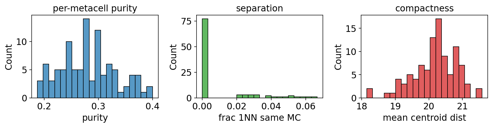
6. Benchmarking metrics (purity / separation / compactness)#
# Compute purity / separation / compactness AND show the 3-panel histogram
# in one call (ov.pl.metacell_metrics returns the per-metacell tables too).
purity, separation, compactness = ov.pl.metacell_metrics(
    mc, label_key='clusters', use_rep='X_pca',
)
7. mcRigor: statistical validation#
# mcRigor's double-permutation null. dubious_rate = fraction of cells in
# heterogeneous metacells; rigor_score = 1 - 0.5*(dubious_rate + zero_rate).
rep = mc.check_rigor(layer_lognorm='lognorm', n_rep=20,
                     feature_use=1000, random_state=0)
print(f'rigor_score : {rep.score:.3f}')
print(f'dubious_rate: {rep.dubious_rate:.3f}')
print(f'zero_rate   : {rep.zero_rate:.3f}')
print(f'# metacells : {rep.n_metacells}')
rigor_score : 0.463
dubious_rate: 1.000
zero_rate   : 0.074
# metacells : 100
7.1 Per-metacell mcDiv vs size#
# mcDiv vs metacell size, overlaid with size-stratified threshold.
ov.pl.rigor_scatter(rep)
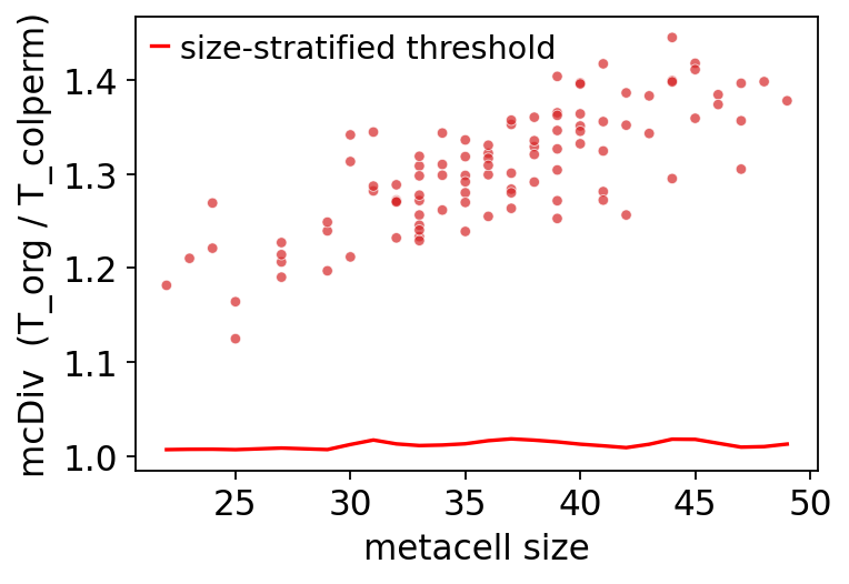
<Axes: xlabel='metacell size', ylabel='mcDiv (T_org / T_colperm)'>
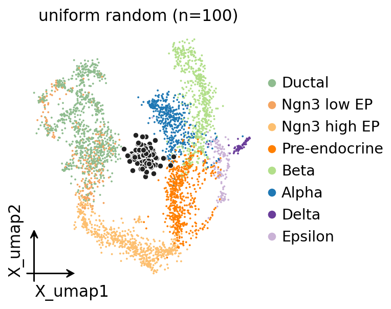
8. UMAP with metacell centroids#
# UMAP coloured by celltype with metacell centroids overlaid in dark grey.
# For uniform random the centroids should be scattered without obvious
# alignment to cell-type clusters.
import matplotlib.pyplot as plt
fig, ax = plt.subplots(figsize=(5, 4))
ov.pl.embedding(mc.adata, basis='X_umap', color='clusters', ax=ax, show=False,
                frameon='small', title='uniform random (n=100)', size=12)
labels = mc._fit_result.assignments
pts = np.array([mc.adata.obsm['X_umap'][labels == u].mean(axis=0)
                for u in np.unique(labels)])
ax.scatter(pts[:, 0], pts[:, 1], s=24, c='#222',
           edgecolors='white', linewidths=0.6, zorder=5)
plt.tight_layout(); plt.show()
9. Per-celltype purity boxplot#
# Per-celltype boxplot of metacell purity.
ov.pl.metacell_purity_box(mc, label_key='clusters')
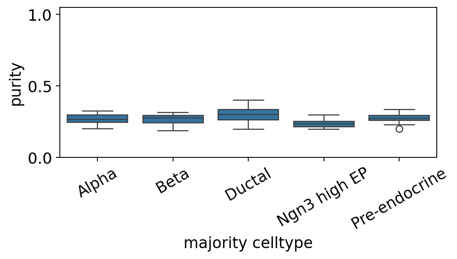
<Axes: xlabel='majority celltype', ylabel='purity'>
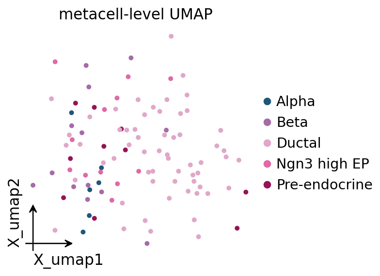
10. Metacell-level UMAP#
# Treat the metacell AnnData as a smaller dataset and run the standard
# omicverse preprocess -> pca -> neighbors -> umap loop on it.
ad_mc = ov.pp.preprocess(ad_mc, mode='shiftlog|pearson',
                          n_HVGs=min(2000, ad_mc.n_vars))
ad_mc = ad_mc[:, ad_mc.var.highly_variable_features]
ov.pp.scale(ad_mc)
ov.pp.pca(ad_mc, layer='scaled', n_pcs=min(30, ad_mc.n_obs - 1))
ad_mc.obsm['X_pca'] = ad_mc.obsm['scaled|original|X_pca']
ov.pp.neighbors(ad_mc, n_neighbors=min(15, ad_mc.n_obs - 1), use_rep='X_pca')
ov.pp.umap(ad_mc)
ov.pl.embedding(ad_mc, basis='X_umap', color='clusters',
                frameon='small', title='metacell-level UMAP', size=80)
🔍 [2026-05-19 18:06:07] Running preprocessing in 'cpu' mode...
Begin robust gene identification
    After filtration, 2000/2000 genes are kept.
    Among 2000 genes, 2000 genes are robust.
✅ Robust gene identification completed successfully.
Begin size normalization: shiftlog and HVGs selection pearson

🔍 Count Normalization:
   Target sum: 500000.0
   Exclude highly expressed: True
   Max fraction threshold: 0.2
   ⚠️ Excluding 0 highly-expressed genes from normalization computation
   Excluded genes: []

✅ Count Normalization Completed Successfully!
   ✓ Processed: 100 cells × 2,000 genes
   ✓ Runtime: 0.00s

🔍 Highly Variable Genes Selection (Experimental):
   Method: pearson_residuals
   Target genes: 2,000
   Theta (overdispersion): 100

✅ Experimental HVG Selection Completed Successfully!
   ✓ Selected: 2,000 highly variable genes out of 2,000 total (100.0%)
   ✓ Results added to AnnData object:
     • 'highly_variable': Boolean vector (adata.var)
     • 'highly_variable_rank': Float vector (adata.var)
     • 'highly_variable_nbatches': Int vector (adata.var)
     • 'highly_variable_intersection': Boolean vector (adata.var)
     • 'means': Float vector (adata.var)
     • 'variances': Float vector (adata.var)
     • 'residual_variances': Float vector (adata.var)
    Time to analyze data in cpu: 0.04 seconds.
✅ Preprocessing completed successfully.
    Added:
        'highly_variable_features', boolean vector (adata.var)
        'means', float vector (adata.var)
        'variances', float vector (adata.var)
        'residual_variances', float vector (adata.var)
        'counts', raw counts layer (adata.layers)
    End of size normalization: shiftlog and HVGs selection pearson

╭─ SUMMARY: preprocess ──────────────────────────────────────────────╮
│  Duration: 0.0464s                                                 │
│  Shape:    100 x 2,000 (Unchanged)                                 │
│                                                                    │
│  CHANGES DETECTED                                                  │
│  ────────────────                                                  │
│  ● UNS    │ ✚ REFERENCE_MANU                                       │
│           │ ✚ _ov_provenance                                       │
│           │ ✚ history_log                                          │
│           │ ✚ hvg                                                  │
│           │ ✚ log1p                                                │
│           │ ✚ status                                               │
│           │ ✚ status_args                                          │
│                                                                    │
│  ● LAYERS │ ✚ counts (sparse matrix, 100x2000)                     │
│                                                                    │
╰────────────────────────────────────────────────────────────────────╯

╭─ SUMMARY: scale ───────────────────────────────────────────────────╮
│  Duration: 0.0133s                                                 │
│  Shape:    100 x 2,000 (Unchanged)                                 │
│                                                                    │
│  CHANGES DETECTED                                                  │
│  ────────────────                                                  │
│  ● LAYERS │ ✚ scaled (array, 100x2000)                             │
│                                                                    │
╰────────────────────────────────────────────────────────────────────╯
computing PCA🔍
    with n_comps=30
   🖥️ Using sklearn PCA for CPU computation
   🖥️ sklearn PCA backend: CPU computation
   📊 PCA input data type: ArrayView, shape: (100, 2000), dtype: float64
🔧 PCA solver used: covariance_eigh
    finished✅ (1.46s)

╭─ SUMMARY: pca ─────────────────────────────────────────────────────╮
│  Duration: 1.4664s                                                 │
│  Shape:    100 x 2,000 (Unchanged)                                 │
│                                                                    │
│  CHANGES DETECTED                                                  │
│  ────────────────                                                  │
│  ● UNS    │ ✚ pca                                                  │
│           │ └─ params: {'zero_center': True, 'use_highly_variable': Tr...│
│           │ ✚ scaled|original|cum_sum_eigenvalues                  │
│           │ ✚ scaled|original|pca_var_ratios                       │
│                                                                    │
│  ● OBSM   │ ✚ X_pca (array, 100x30)                                │
│           │ ✚ scaled|original|X_pca (array, 100x30)                │
│                                                                    │
╰────────────────────────────────────────────────────────────────────╯
🖥️ Using Scanpy CPU to calculate neighbors...

🔍 K-Nearest Neighbors Graph Construction:
   Mode: cpu
   Neighbors: 15
   Method: umap
   Metric: euclidean
   Representation: X_pca
   🔍 Computing neighbor distances...
   🔍 Computing connectivity matrix...
   💡 Using UMAP-style connectivity
   ✓ Graph is fully connected

✅ KNN Graph Construction Completed Successfully!
   ✓ Processed: 100 cells with 15 neighbors each
   ✓ Results added to AnnData object:
     • 'neighbors': Neighbors metadata (adata.uns)
     • 'distances': Distance matrix (adata.obsp)
     • 'connectivities': Connectivity matrix (adata.obsp)

╭─ SUMMARY: neighbors ───────────────────────────────────────────────╮
│  Duration: 0.0867s                                                 │
│  Shape:    100 x 2,000 (Unchanged)                                 │
│                                                                    │
│  CHANGES DETECTED                                                  │
│  ────────────────                                                  │
│  ● UNS    │ ✚ neighbors                                            │
│           │ └─ params: {'n_neighbors': 15, 'method': 'umap', 'random_s...│
│                                                                    │
│  ● OBSP   │ ✚ connectivities (sparse matrix, 100x100)              │
│           │ ✚ distances (sparse matrix, 100x100)                   │
│                                                                    │
╰────────────────────────────────────────────────────────────────────╯
🔍 [2026-05-19 18:06:08] Running UMAP in 'cpu' mode...
🖥️ Using Scanpy CPU UMAP...

🔍 UMAP Dimensionality Reduction:
   Mode: cpu
   Method: umap
   Components: 2
   Min distance: 0.5
{'n_neighbors': 15, 'method': 'umap', 'random_state': 0, 'metric': 'euclidean', 'use_rep': 'X_pca'}
   🔍 Computing UMAP parameters...
   🔍 Computing UMAP embedding (classic method)...

✅ UMAP Dimensionality Reduction Completed Successfully!
   ✓ Embedding shape: 100 cells × 2 dimensions
   ✓ Results added to AnnData object:
     • 'X_umap': UMAP coordinates (adata.obsm)
     • 'umap': UMAP parameters (adata.uns)
✅ UMAP completed successfully.

╭─ SUMMARY: umap ────────────────────────────────────────────────────╮
│  Duration: 0.013s                                                  │
│  Shape:    100 x 2,000 (Unchanged)                                 │
│                                                                    │
│  CHANGES DETECTED                                                  │
│  ────────────────                                                  │
│  ● UNS    │ ✚ umap                                                 │
│           │ └─ params: {'a': 0.5830300199950147, 'b': 1.334166993228519}│
│                                                                    │
│  ● OBSM   │ ✚ X_umap (array, 100x2)                                │
│                                                                    │
╰────────────────────────────────────────────────────────────────────╯
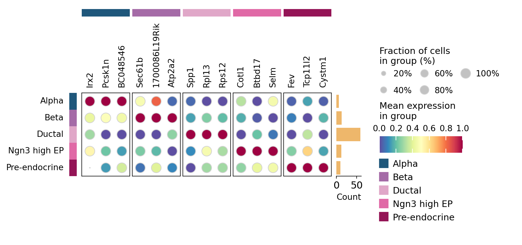
11. Top markers per celltype on the metacell AnnData#
# Find top markers per celltype on the metacell AnnData (omicverse helper —
# drops the categories with <2 metacells automatically and reports cell-type
# fractions ``pts`` along with the gene names).
counts = ad_mc.obs['clusters'].value_counts()
keep = counts[counts >= 2].index.tolist()
ad_mc_for_de = ad_mc[ad_mc.obs['clusters'].isin(keep)].copy()
ad_mc_for_de.obs['clusters'] = ad_mc_for_de.obs['clusters'].astype('category')

ov.single.find_markers(ad_mc_for_de, groupby='clusters', method='wilcoxon',
                       key_added='rank_genes_groups', pts=True, use_gpu=False)
ov.single.get_markers(ad_mc_for_de, n_genes=3, key='rank_genes_groups')
🔍 Finding marker genes | method: wilcoxon | groupby: clusters | n_groups: 5 | n_genes: 50
✅ Done | 5 groups × 50 genes | corr: benjamini-hochberg | stored in adata.uns['rank_genes_groups']
| group | rank | names | scores | logfoldchanges | pvals | pvals_adj | pct_group | pct_rest | |
|---|---|---|---|---|---|---|---|---|---|
| 0 | Alpha | 1 | Irx2 | 3.788182 | 1.544677 | 1.517534e-04 | 0.100786 | 1.0 | 0.989362 |
| 1 | Alpha | 2 | Pcsk1n | 3.701098 | 0.617851 | 2.146687e-04 | 0.100786 | 1.0 | 1.000000 |
| 2 | Alpha | 3 | BC048546 | 3.570471 | 0.936704 | 3.563401e-04 | 0.100786 | 1.0 | 1.000000 |
| 3 | Beta | 1 | Sec61b | 4.371371 | 0.295734 | 1.234688e-05 | 0.020171 | 1.0 | 1.000000 |
| 4 | Beta | 2 | 1700086L19Rik | 4.227880 | 0.545602 | 2.359042e-05 | 0.020171 | 1.0 | 1.000000 |
| 5 | Beta | 3 | Atp2a2 | 4.115136 | 0.843974 | 3.869513e-05 | 0.020171 | 1.0 | 1.000000 |
| 6 | Ductal | 1 | Spp1 | 5.778334 | 0.377293 | 7.544381e-09 | 0.000012 | 1.0 | 1.000000 |
| 7 | Ductal | 2 | Rpl13 | 5.371853 | 0.110457 | 7.793141e-08 | 0.000026 | 1.0 | 1.000000 |
| 8 | Ductal | 3 | Rps12 | 5.217671 | 0.150540 | 1.811868e-07 | 0.000047 | 1.0 | 1.000000 |
| 9 | Ngn3 high EP | 1 | Cotl1 | 4.433781 | 0.426164 | 9.259459e-06 | 0.018519 | 1.0 | 1.000000 |
| 10 | Ngn3 high EP | 2 | Btbd17 | 4.030710 | 0.522891 | 5.560857e-05 | 0.055609 | 1.0 | 1.000000 |
| 11 | Ngn3 high EP | 3 | Selm | 3.776139 | 0.364340 | 1.592781e-04 | 0.078716 | 1.0 | 1.000000 |
| 12 | Pre-endocrine | 1 | Fev | 4.412045 | 0.809875 | 1.023990e-05 | 0.020480 | 1.0 | 1.000000 |
| 13 | Pre-endocrine | 2 | Tcp11l2 | 3.986926 | 0.918744 | 6.693494e-05 | 0.059289 | 1.0 | 1.000000 |
| 14 | Pre-endocrine | 3 | Cystm1 | 3.895008 | 0.274352 | 9.819540e-05 | 0.059289 | 1.0 | 1.000000 |
# Dotplot of top markers per metacell-level celltype.
ov.pl.markers_dotplot(ad_mc_for_de, groupby='clusters', n_genes=3,
                      key='rank_genes_groups')
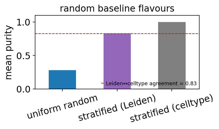
12. Stratification leakage: why “Leiden-stratified random” is misleading#
Three “random” flavours on this dataset:
uniform (the primary baseline above) — mean purity should be near the largest celltype’s proportion.
stratified by Leiden — each metacell stays inside one Leiden community. On this dataset Leiden (resolution = 0.8) has 13 clusters and a mean Leiden-vs-celltype agreement of ~0.83, so this baseline inherits 83 % of the celltype signal for free. Not a real baseline.
stratified by celltype — full tautology, mean purity = 1.0.
This is dataset-dependent — on a dataset where Leiden doesn’t already track celltype (heavy batch effects, very rare populations), Leiden-stratified random would be a fairer comparison. Always inspect the Leiden ↔ celltype contingency before trusting it as a baseline.
# Three random flavours + the Leiden-vs-celltype contingency that explains
# why "stratified by Leiden" cheats on this dataset.
mc_strat_leiden = ov.single.MetaCell(
    adata.copy(), method='random', n_metacells=100,
    stratify_key='leiden', random_state=0,
).fit()
mc_strat_celltype = ov.single.MetaCell(
    adata.copy(), method='random', n_metacells=100,
    stratify_key='clusters', random_state=0,
).fit()

p_uniform   = mc.compute_purity('clusters').purity.mean()
p_leiden    = mc_strat_leiden.compute_purity('clusters').purity.mean()
p_strat_ct  = mc_strat_celltype.compute_purity('clusters').purity.mean()

# Quick Leiden-vs-celltype agreement: how much celltype info does Leiden encode?
ct = pd.crosstab(adata.obs['leiden'], adata.obs['clusters'])
leiden_purity = (ct.max(axis=1) / ct.sum(axis=1)).mean()

print(f'mean Leiden-vs-celltype agreement: {leiden_purity:.3f}')
print()
print(f'uniform random            : mean purity = {p_uniform:.3f}  (the honest floor)')
print(f'stratified by Leiden      : mean purity = {p_leiden:.3f}  (leaks {leiden_purity:.0%} of celltype info)')
print(f'stratified by celltype    : mean purity = {p_strat_ct:.3f}  (tautology)')
mean Leiden-vs-celltype agreement: 0.827

uniform random            : mean purity = 0.282  (the honest floor)
stratified by Leiden      : mean purity = 0.832  (leaks 83% of celltype info)
stratified by celltype    : mean purity = 1.000  (tautology)
# Bar chart comparing the three flavours — note that the Leiden bar tracks
# the Leiden-vs-celltype agreement (red dashed), not real metacell quality.
import matplotlib.pyplot as plt
fig, ax = plt.subplots(figsize=(5, 3))
pd.Series({
    'uniform random': p_uniform,
    'stratified (Leiden)': p_leiden,
    'stratified (celltype)': p_strat_ct,
}).plot.bar(ax=ax, color=['#1f77b4', '#9467bd', '#7f7f7f'])
ax.axhline(leiden_purity, color='red', linestyle='--', linewidth=1,
           label=f'Leiden↔celltype agreement = {leiden_purity:.2f}')
ax.set_ylabel('mean purity'); ax.set_ylim(0, 1.1)
ax.set_title('random baseline flavours')
ax.tick_params(axis='x', rotation=15)
ax.legend(loc='lower right', fontsize=8)
plt.tight_layout(); plt.show()
13. Save / load roundtrip#
# Save/load roundtrip — every backend supports this.
import tempfile, os
with tempfile.NamedTemporaryFile(suffix='.pkl', delete=False) as f:
    path = f.name
mc.save(path)

mc2 = ov.single.MetaCell(adata.copy(), method='random', n_metacells=100,
                          use_rep='X_pca', random_state=0)
mc2.load(path)
print(f'saved+loaded {path}')
os.remove(path)
saved+loaded /tmp/tmpmhyc7skr.pkl
14. Takeaways#
Uniform random is the honest baseline. On this pancreas dataset it gives mean purity ≈ 0.28 — roughly the largest celltype’s relative size. Any principled metacell method must beat this.
Do not use
stratify_key='leiden'as a baseline unless you’ve checked that Leiden ↔ celltype agreement is low on your data. Here it’s 0.83, so Leiden-stratified random looks deceptively good (also ~0.83) because Leiden already encodes the celltype structure.Stratifying by the evaluation label (
clusters→ celltype) is a strict tautology — purity = 1.0. Only useful to sanity-check that purity computation works at all.A working pipeline should show:
uniform_random << kmeans < seacells / metaq. In this notebook’s run that’s roughly0.28 < 0.83 ≤ 0.86, which means the principled methods are ~3× better than random — earning their complexity.