Analyze Xenium data

The 10x Genomics Xenium In Situ platform is an image-based in situ technology that reports counts of a pre-designed gene panel at single-cell resolution. A single Xenium experiment produces a stitched tissue region in microns, per-cell centroids and polygon boundaries, individual transcript locations, and multi-channel morphology images. It is widely used for tumor microenvironment studies, brain atlasing, and validation of dissociated single-cell data.

This tutorial mirrors the Nanostring CosMx tutorial (t_nanostring_preprocess.ipynb) and is informed by squidpy’s Xenium vignette. We use ov.io.read_xenium() and a standard Leiden-based downstream analysis (skipping CAST). Key outputs you will see:

• ov.io.read_xenium() parsing the 10x outs/ layout into an AnnData with spatial coordinates in microns and cell polygon boundaries as WKT strings on obs['geometry']

• basic per-cell QC against control probes / codewords

• the standard OmicVerse preprocessing pipeline (normalize_total → log1p → scale → pca)

• k-NN graph + Leiden clustering

• spatial visualization of the clusters over the tissue layout via both ov.pl.embedding (centroid scatter) and ov.pl.spatialseg (polygon overlay)

1. Environment setup

Import omicverse, set the plotting style, and enable auto-reload. ov.style(font_path='Arial') keeps exported figures consistent across platforms.

from pathlib import Path
import numpy as np
import omicverse as ov
ov.style(font_path='Arial')

%load_ext autoreload
%autoreload 2

🔬 Starting plot initialization...
Using already downloaded Arial font from: /tmp/omicverse_arial.ttf
Registered as: Arial
🧬 Detecting GPU devices…
✅ NVIDIA CUDA GPUs detected: 1
    • [CUDA 0] NVIDIA H100 80GB HBM3
      Memory: 79.1 GB | Compute: 9.0

   ____            _     _    __                  
  / __ \____ ___  (_)___| |  / /__  _____________ 
 / / / / __ `__ \/ / ___/ | / / _ \/ ___/ ___/ _ \ 
/ /_/ / / / / / / / /__ | |/ /  __/ /  (__  )  __/ 
\____/_/ /_/ /_/_/\___/ |___/\___/_/  /____/\___/                                              

🔖 Version: 2.1.2rc1   📚 Tutorials: https://omicverse.readthedocs.io/
✅ plot_set complete.

ov.settings.cpu_gpu_mixed_init()

CPU-GPU mixed mode activated
Available GPU accelerators: CUDA

2. Download the Xenium dataset

We use the public Xenium FFPE Human Breast Cancer Replicate 1 sample from 10x (≈167k cells, 313 genes, Breast Cancer Tumor Microenvironment panel + 33 custom targets). The full outs bundle is several GB because of the multi-channel morphology OME-TIFFs, but the minimum files for a Leiden analysis with segmentation visualization are only ~40 MB:

• cell_feature_matrix.h5 — sparse gene × cell counts (≈12 MB)

• cells.csv.gz — per-cell metadata including x_centroid, y_centroid in microns (≈8 MB)

• cell_boundaries.parquet — per-cell polygon vertices for ov.pl.spatialseg (≈8 MB)

• experiment.xenium — run metadata (JSON)

If you also want the H&E / DAPI background overlay, download morphology_focus.ome.tif (≈624 MB) and call ov.io.read_xenium(..., load_image=True).

# !mkdir -p data/xenium_breast_rep1
# BASE='https://cf.10xgenomics.com/samples/xenium/1.0.1/Xenium_FFPE_Human_Breast_Cancer_Rep1'
# !wget -O data/xenium_breast_rep1/cell_feature_matrix.h5  $BASE/Xenium_FFPE_Human_Breast_Cancer_Rep1_cell_feature_matrix.h5
# !wget -O data/xenium_breast_rep1/cells.csv.gz            $BASE/Xenium_FFPE_Human_Breast_Cancer_Rep1_cells.csv.gz
# !wget -O data/xenium_breast_rep1/cell_boundaries.parquet $BASE/Xenium_FFPE_Human_Breast_Cancer_Rep1_cell_boundaries.parquet
# !wget -O data/xenium_breast_rep1/experiment.xenium       $BASE/Xenium_FFPE_Human_Breast_Cancer_Rep1_experiment.xenium
# Optional — ~624 MB, only needed for a morphology background in ov.pl.spatial:
# !wget -O data/xenium_breast_rep1/morphology_focus.ome.tif $BASE/Xenium_FFPE_Human_Breast_Cancer_Rep1_morphology_focus.ome.tif

sample_dir = Path('data') / 'xenium_breast_rep1'
ov.utils.print_tree(sample_dir)

xenium_breast_rep1/
├── cell_boundaries.parquet
├── cell_feature_matrix.h5
├── cells.csv.gz
├── experiment.xenium
└── morphology_focus.ome.tif

3. Read the Xenium dataset

ov.io.read_xenium() handles the 10x outs/ layout:

• reads cell_feature_matrix.h5 via the 10x HDF5 parser

• drops non-Gene-Expression features (control probes / codewords) so downstream PCA and HVG don’t waste capacity

• merges cells.csv.gz (or cells.parquet) into obs

• writes cell centroids in microns to obsm['spatial']

• converts cell_boundaries.parquet vertex vectors into per-cell WKT POLYGON strings on obs['geometry'] — the format expected by ov.pl.spatialseg

• sets uns['spatial'][library_id]['scalefactors'] (tissue_hires_scalef = 1 / pixel_size) so micron coordinates map correctly into image-pixel space when a morphology image is loaded

• parses experiment.xenium into uns['spatial'][library_id]['metadata']

Pass load_image=False to skip the (large) morphology OME-TIFF, and load_boundaries=False to skip polygon extraction.

adata = ov.io.read_xenium(sample_dir, load_image=False)
adata

[Xenium] Reading Xenium data from: /scratch/users/steorra/xenium_test/breast_rep1
[Xenium] Loaded cell polygons (geometry WKT) for 167780/167780 cells
[Xenium] Done (n_obs=167780, n_vars=313, library_id=Replicate 1)

AnnData object with n_obs × n_vars = 167780 × 313
    obs: 'transcript_counts', 'control_probe_counts', 'control_codeword_counts', 'total_counts', 'cell_area', 'nucleus_area', 'geometry'
    var: 'gene_ids', 'feature_types', 'genome'
    uns: 'spatial', 'omicverse_io'
    obsm: 'spatial'

library_id = next(iter(adata.uns['spatial']))
sf = adata.uns['spatial'][library_id]['scalefactors']
print('library_id          :', library_id)
print('spatial range (µm)  :',
      adata.obsm['spatial'].min(axis=0).tolist(), '->',
      adata.obsm['spatial'].max(axis=0).tolist())
print('pixel size (µm/px)  :', 1 / sf['tissue_hires_scalef'])
print('mean cell diameter :', round(sf['spot_diameter_fullres'] / sf['tissue_hires_scalef'], 2), 'µm')
print('cells with geometry:', (adata.obs['geometry'] != '').sum())

library_id          : Replicate 1
spatial range (µm)  : [2.1325161457061768, 3.642256736755371] -> [7523.0869140625, 5474.37939453125]
pixel size (µm/px)  : 0.2125
mean cell diameter : 15.7 µm
cells with geometry: 164000

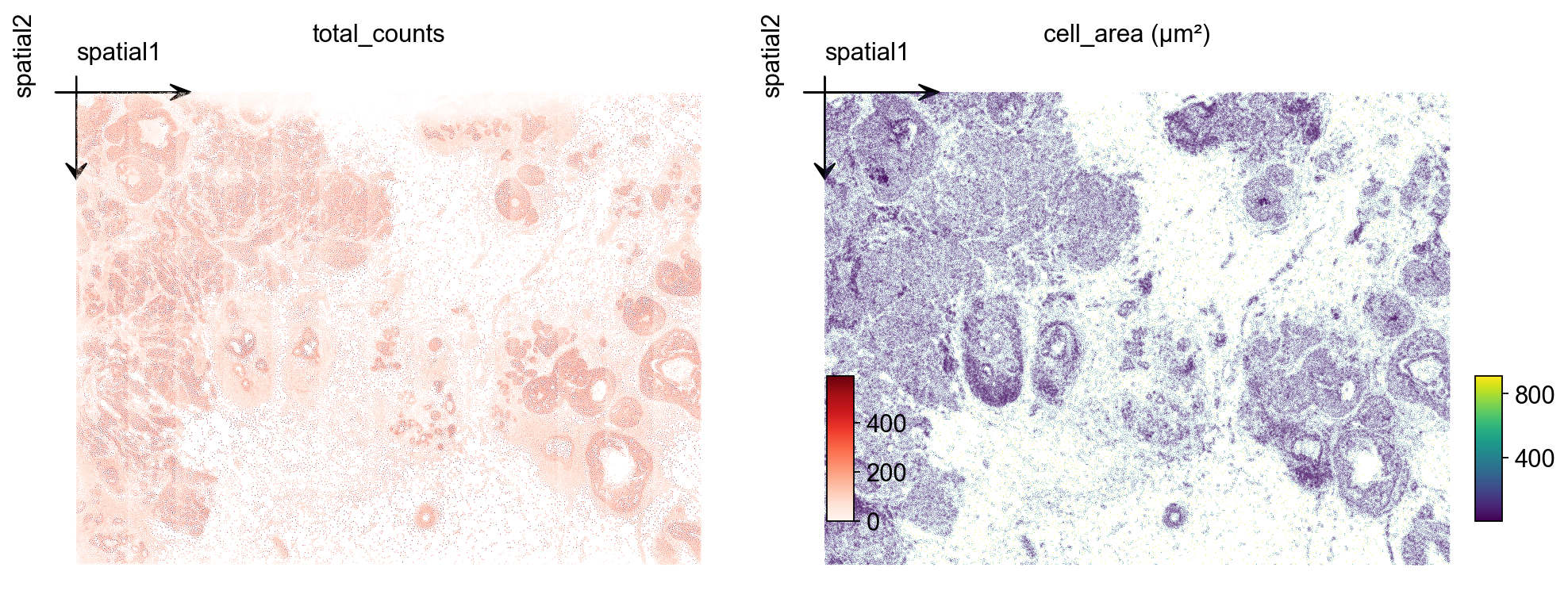
4. Inspect spatial QC

Two quick checks over the tissue layout: total_counts per cell and cell_area (in square microns). For a tumor microenvironment section you typically see counts concentrated on epithelial / tumor tiles and a roughly bimodal area distribution (small immune vs. large epithelial).

import matplotlib.pyplot as plt
fig, axs = plt.subplots(1, 2, figsize=(12, 5))
ov.pl.embedding(
    adata, basis='spatial', color='total_counts',
    vmax='p99', cmap='Reds', ax=axs[0], show=False, title='total_counts',
)
axs[0].invert_yaxis()
ov.pl.embedding(
    adata, basis='spatial', color='cell_area',
    vmax='p99', cmap='viridis', ax=axs[1], show=False, title='cell_area (µm²)',
)
axs[1].invert_yaxis()
plt.tight_layout()

5. Cell-level QC

Filter out cells with very low transcript counts — these are usually segmentation artifacts or empty nuclei. A threshold of 10 counts is mild; tune based on the total_counts histogram.

import scipy.sparse as sp
counts = np.asarray(adata.X.sum(axis=1)).ravel() if sp.issparse(adata.X) else adata.X.sum(axis=1)
print(f'cells pre-QC : {adata.n_obs}')
adata = adata[counts >= 10].copy()
print(f'cells post-QC: {adata.n_obs} (>= 10 transcripts/cell)')

cells pre-QC : 167780
cells post-QC: 164000 (>= 10 transcripts/cell)

6. Normalize, log-transform and scale

We use the standard normalize_total + log1p + scale pipeline. Because the panel is small (313 genes), we skip HVG selection and use all genes for PCA.

ov.pp.normalize_total(adata, target_sum=1e4)
ov.pp.log1p(adata)
ov.pp.scale(adata)

🔍 Count Normalization:
   Target sum: 10000.0
   Exclude highly expressed: False

✅ Count Normalization Completed Successfully!
   ✓ Processed: 164,000 cells × 313 genes
   ✓ Runtime: 0.04s
╭─ SUMMARY: scale ───────────────────────────────────────────────────╮
│  Duration: 0.7115s                                                 │
│  Shape:    164,000 x 313 (Unchanged)                               │
│                                                                    │
│  CHANGES DETECTED                                                  │
│  ────────────────                                                  │
│  ● UNS    │ ✚ REFERENCE_MANU                                       │
│           │ ✚ status                                               │
│           │ ✚ status_args                                          │
│                                                                    │
│  ● LAYERS │ ✚ scaled (array, 164000x313)                           │
│                                                                    │
╰────────────────────────────────────────────────────────────────────╯

7. PCA + neighbors + Leiden

Compute the first 50 principal components of the scaled matrix, build a k-NN graph, and run Leiden. For a 164k-cell Xenium section, resolution=0.5 typically gives 10–20 clusters mapping to broad tissue structure. Push higher for finer subtypes, lower for compartments.

ov.pp.pca(adata, layer='scaled', n_pcs=50)
ov.pp.neighbors(
    adata, n_neighbors=15,
    use_rep='scaled|original|X_pca', n_pcs=50,
)
ov.pp.leiden(adata, resolution=0.5)
print(f"leiden: {adata.obs['leiden'].nunique()} clusters")

🚀 Using GPU to calculate PCA...
NVIDIA CUDA GPUs detected:
📊 [CUDA 0] NVIDIA H100 80GB HBM3
    ------------------------------ 5/81559 MiB (0.0%)
computing PCA🔍
    with n_comps=50

Using CUDA device: NVIDIA H100 80GB HBM3
✅ Using built-in torch_pca for GPU-accelerated PCA
   🚀 Using torch_pca PCA for CUDA GPU acceleration
   🚀 torch_pca PCA backend: CUDA GPU acceleration (supports sparse matrices)
   📊 PCA input data type: ndarray, shape: (164000, 313), dtype: float64
   🔧 solver_used_in_uns (planned): covariance_eigh
🔧 PCA solver used: covariance_eigh
    finished✅ (0.56s)

╭─ SUMMARY: pca ─────────────────────────────────────────────────────╮
│  Duration: 0.5841s                                                 │
│  Shape:    164,000 x 313 (Unchanged)                               │
│                                                                    │
│  CHANGES DETECTED                                                  │
│  ────────────────                                                  │
│  ● UNS    │ ✚ pca                                                  │
│           │ └─ params: {'zero_center': True, 'use_highly_variable': Fa...│
│           │ ✚ scaled|original|cum_sum_eigenvalues                  │
│           │ ✚ scaled|original|pca_var_ratios                       │
│                                                                    │
│  ● OBSM   │ ✚ X_pca (array, 164000x50)                             │
│           │ ✚ scaled|original|X_pca (array, 164000x50)             │
│                                                                    │
╰────────────────────────────────────────────────────────────────────╯
🚀 Using torch CPU/GPU mixed mode to calculate neighbors...
NVIDIA CUDA GPUs detected:
📊 [CUDA 0] NVIDIA H100 80GB HBM3
    ------------------------------ 1487/81559 MiB (1.8%)
🚀 Mixed mode default transformer: pyg

🔍 K-Nearest Neighbors Graph Construction:
   Mode: cpu-gpu-mixed
   Neighbors: 15
   Method: torch
   Metric: euclidean
   Transformer: pyg
   Representation: scaled|original|X_pca
   PCs used: 50
   🔍 Computing neighbor distances...
   💡 Using PyTorch Geometric KNN on cuda
🔍 Computing connectivity matrix...
   💡 Using UMAP-style connectivity
✓ Graph is fully connected

✅ KNN Graph Construction Completed Successfully!
   ✓ Processed: 164,000 cells with 15 neighbors each
   ✓ Results added to AnnData object:
     • 'neighbors': Neighbors metadata (adata.uns)
     • 'distances': Distance matrix (adata.obsp)
     • 'connectivities': Connectivity matrix (adata.obsp)

╭─ SUMMARY: neighbors ───────────────────────────────────────────────╮
│  Duration: 12.3926s                                                │
│  Shape:    164,000 x 313 (Unchanged)                               │
│                                                                    │
│  CHANGES DETECTED                                                  │
│  ────────────────                                                  │
│  ● UNS    │ ✚ neighbors                                            │
│           │ └─ params: {'n_neighbors': 15, 'method': 'torch', 'random_...│
│                                                                    │
│  ● OBSP   │ ✚ connectivities (sparse matrix, 164000x164000)        │
│           │ ✚ distances (sparse matrix, 164000x164000)             │
│                                                                    │
╰────────────────────────────────────────────────────────────────────╯
⚙️ Using torch CPU/GPU mixed mode to calculate Leiden...
NVIDIA CUDA GPUs detected:
📊 [CUDA 0] NVIDIA H100 80GB HBM3
    |----------------------------- 2943/81559 MiB (3.6%)
Using batch size `n_batches` calculated from sqrt(n_obs): 404
╭─ SUMMARY: leiden ──────────────────────────────────────────────────╮
│  Duration: 158.7248s                                               │
│  Shape:    164,000 x 313 (Unchanged)                               │
│                                                                    │
│  CHANGES DETECTED                                                  │
│  ────────────────                                                  │
│  ● OBS    │ ✚ leiden (category)                                    │
│                                                                    │
│  ● UNS    │ ✚ leiden                                               │
│           │ └─ params: {'resolution': 0.5, 'random_state': 0, 'local_i...│
│                                                                    │
╰────────────────────────────────────────────────────────────────────╯
leiden: 20 clusters

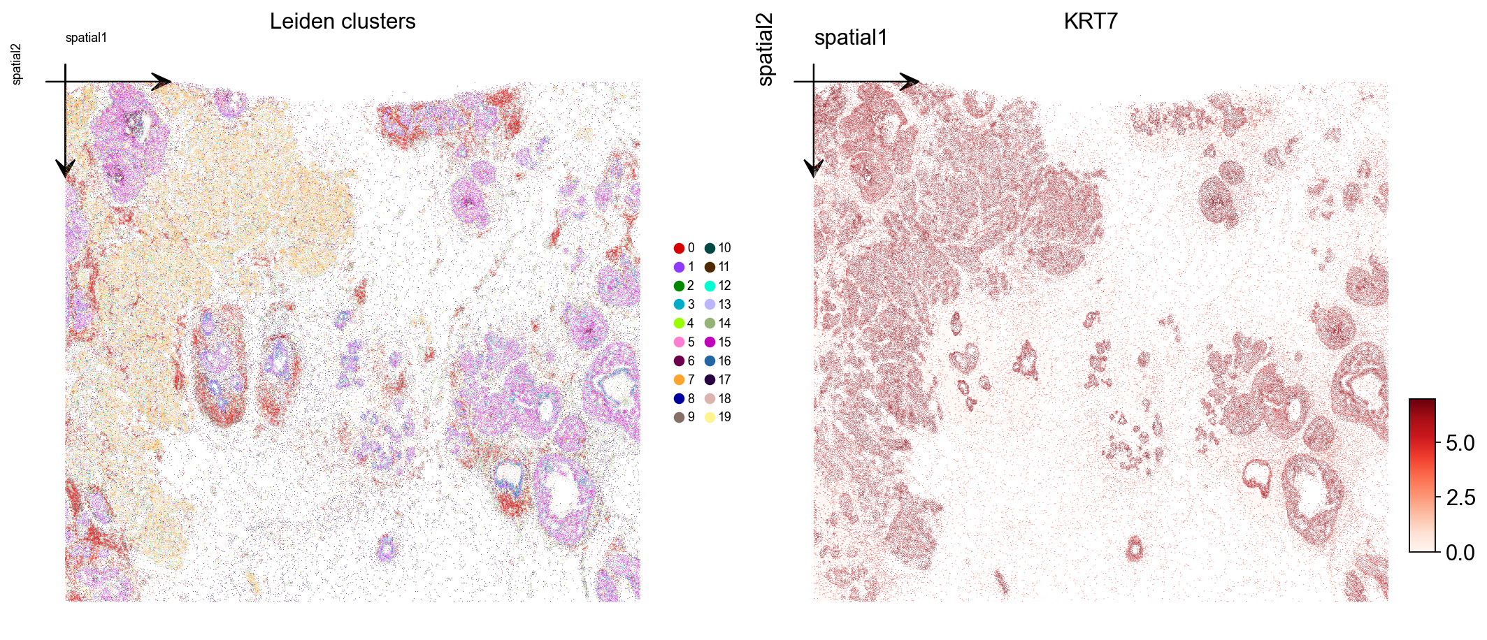
8. Visualize Leiden clusters on the tissue

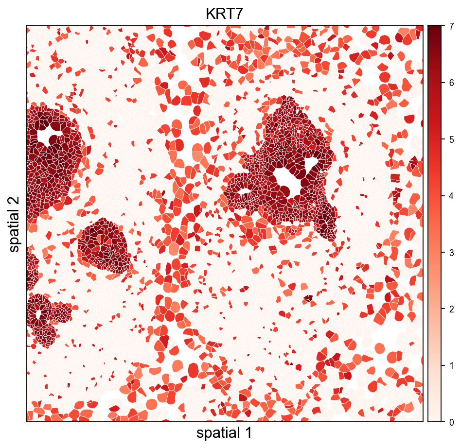
Plot the Leiden label and one marker gene over the spatial layout. Xenium centroids are in image-pixel convention (y grows downward); ax.invert_yaxis() lines the plot up with the tissue image you would overlay in step 10.

marker = next((g for g in ['KRT7', 'EPCAM', 'ERBB2', 'ESR1', 'KRT14']
               if g in adata.var_names), adata.var_names[0])

fig, axs = plt.subplots(1, 2, figsize=(13, 6))
ov.pl.embedding(
    adata, basis='spatial', color='leiden',
    palette=ov.pl.palette_112,
    legend_fontsize=8, ax=axs[0], show=False, title='Leiden clusters',
)
axs[0].invert_yaxis()
ov.pl.embedding(
    adata, basis='spatial', color=marker,
    vmax='p99.2', cmap='Reds', ax=axs[1], show=False, title=marker,
)
axs[1].invert_yaxis()
plt.tight_layout()

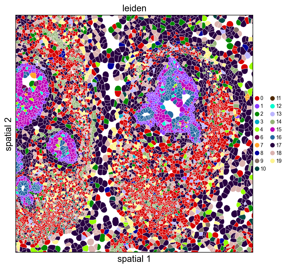
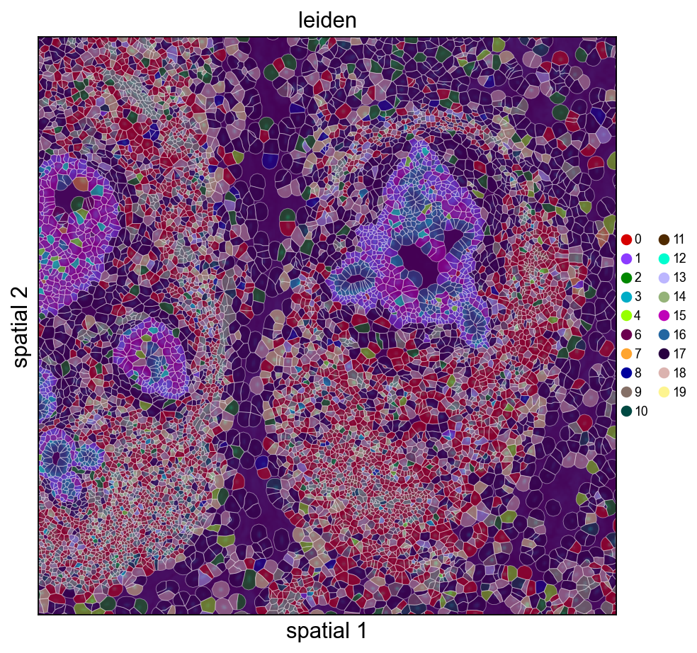
9. Visualize with cell polygons (ov.pl.spatialseg)

Unlike centroid scatter, ov.pl.spatialseg draws each cell as its actual segmented polygon. This is the right view for inspecting cluster boundaries against tissue morphology and for diagnosing oversegmentation.

On a 160k-cell section rendering every polygon produces a dense figure. To see the segmentation itself we also provide a cropped view (crop_coord=(x0, x1, y0, y1) in microns). Pick a region where tumor and stromal compartments should meet — for this breast sample, coordinates around (2000–3200 µm × 2500–3700 µm) land on a mixed compartment.

Rendering every cell polygon for the full 160k-cell section can take minutes and produce a dense image where individual cells aren’t visible. We’ll keep the full-section view to ov.pl.embedding (centroid scatter) and use ov.pl.spatialseg only on a cropped region, where the polygons are actually readable.

ov.pl.spatialseg(
    adata, color='leiden',
    library_id=library_id,
    edges_color='white', edges_width=0.3,
    alpha=1.0, legend_fontsize=8,
    palette=ov.pl.palette_112,
    crop_coord=(2000, 3200, 2500, 3700),
    figsize=(7, 6),
)

<Axes: title={'center': 'leiden'}, xlabel='spatial 1', ylabel='spatial 2'>

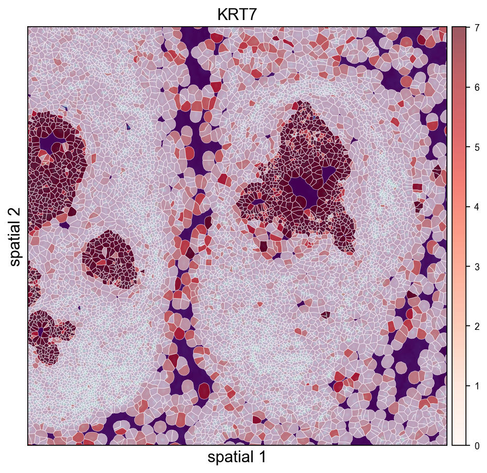
The same view coloured by a tumor-associated marker shows which polygons actually express it — useful for validating that a Leiden cluster and a gene signature agree.

import numpy as np
expr = adata[:, marker].X.toarray().ravel() if hasattr(adata[:, marker].X, 'toarray') else np.asarray(adata[:, marker].X).ravel()
vmax_marker = float(np.percentile(expr[expr > 0], 99)) if (expr > 0).any() else 1.0

ov.pl.spatialseg(
    adata, color=marker,
    library_id=library_id,
    edges_color='white', edges_width=0.3,
    alpha=1.0, legend_fontsize=8,
    cmap='Reds', vmax=vmax_marker,
    crop_coord=(2000, 3200, 2500, 3700),
    figsize=(7, 6),
)

<Axes: title={'center': 'KRT7'}, xlabel='spatial 1', ylabel='spatial 2'>

10. (Optional) overlay on the morphology image

If you downloaded morphology_focus.ome.tif into sample_dir, re-read with load_image=True and use ov.pl.spatial / ov.pl.spatialseg to overlay labels on the morphology background. read_xenium() sets tissue_hires_scalef = 1 / pixel_size so spot coordinates land in image-pixel space.

adata_img = ov.io.read_xenium(sample_dir, load_image=True)
adata_img.obs['leiden'] = adata.obs['leiden']   # carry over labels
ov.pl.spatialseg(
    adata_img, color='leiden', library_id=library_id,
    alpha_img=0.5, alpha=0.8,
    palette=ov.pl.palette_112,
    crop_coord=(2000, 3200, 2500, 3700),
)

For large Xenium sections (cm-scale), always prefer crop_coord=(x0, x1, y0, y1) in microns to zoom into a region — rendering every polygon for the full tissue can take minutes.

11. Save the processed object

Persist the analyzed AnnData so you can skip preprocessing next time. The WKT strings in obs['geometry'] round-trip through adata.write() unchanged.

adata.write('data/xenium_breast_rep1_processed.h5ad')

#adata=ov.read('data/xenium_breast_rep1_processed.h5ad')

12. Cache the loaded AnnData for fast re-reads

Parsing cell_feature_matrix.h5 + cells.csv.gz + cell_boundaries.parquet (including the per-cell WKT polygon construction) takes a few seconds the first time. Pass cache_file= to read_xenium() to write an h5ad snapshot alongside the outs folder — subsequent calls with the same cache_file skip all the parsing and just read the h5ad back, typically ~30× faster.

The cache includes everything: counts, obs/var, spatial coords, polygon WKT strings, image payloads, and experiment metadata. Delete the cache file to force a re-read after updating any of the source files.

import time, os

cache_path = 'data/xenium_breast_rep1_cache.h5ad'
if os.path.exists(cache_path):
    os.remove(cache_path)  # start fresh to show the timing difference

t0 = time.time()
_ = ov.io.read_xenium(sample_dir, load_image=False, cache_file=cache_path)
t_cold = time.time() - t0

t0 = time.time()
_ = ov.io.read_xenium(sample_dir, cache_file=cache_path)
t_warm = time.time() - t0

print(f'cold (raw parse + cache write): {t_cold:.2f} s')
print(f'warm (cache read)              : {t_warm:.2f} s')
print(f'speedup                        : {t_cold / t_warm:.1f}x')

[Xenium] Reading Xenium data from: /scratch/users/steorra/xenium_test/breast_rep1
[Xenium] Loaded cell polygons (geometry WKT) for 167780/167780 cells
[Xenium] Wrote cache AnnData to: /scratch/users/steorra/analysis/omicverse_dev/omicverse/omicverse_guide/docs/Tutorials-space/data/xenium_breast_rep1_cache.h5ad
[Xenium] Done (n_obs=167780, n_vars=313, library_id=Replicate 1)
[Xenium] Reading cached AnnData from: /scratch/users/steorra/analysis/omicverse_dev/omicverse/omicverse_guide/docs/Tutorials-space/data/xenium_breast_rep1_cache.h5ad
cold (raw parse + cache write): 9.70 s
warm (cache read)              : 0.27 s
speedup                        : 35.9x

13. Overlay Leiden clusters on the morphology image

When morphology_focus.ome.tif sits next to the cell_feature_matrix.h5, pass load_image=True and ov.pl.spatialseg will render cell polygons on top of the morphology background. The OME-TIFF is a multi-resolution pyramid (8 levels from 25K×35K down to 201×276), so we only read one level: image_max_dim=4096 picks the highest pyramid level whose largest dimension fits under 4096 px (~1611×2213 for this sample, ~7 MB as uint16, <1 s to load). That is the Xenium analogue of Visium’s hires.png — no need to touch the 25K×35K full-resolution data.

The loader rescales tissue_hires_scalef to the chosen pyramid level, so micron coordinates land on the downsampled image without any extra math on your side.

# One-time call: loads the image, composes the full AnnData, writes the cache
adata_img = ov.io.read_xenium(
    sample_dir,
    load_image=True,
    image_max_dim=4096,
    cache_file='data/xenium_breast_rep1_with_image_cache.h5ad',
)
# Carry Leiden labels from the already-processed adata so we can visualise
# clusters without re-running the pipeline on the image-backed copy.
adata_img = adata_img[adata.obs_names].copy()
adata_img.obs['leiden'] = adata.obs['leiden'].values
img = adata_img.uns['spatial'][library_id]['images']['hires']
sf  = adata_img.uns['spatial'][library_id]['scalefactors']
print('image shape     :', img.shape, 'dtype:', img.dtype)
print('hires_scalef    :', round(sf['tissue_hires_scalef'], 4),
      '(micron -> image-pixel)')
print('fullres diameter:', round(sf['spot_diameter_fullres'], 2), 'px')

[Xenium] Reading cached AnnData from: /scratch/users/steorra/analysis/omicverse_dev/omicverse/omicverse_guide/docs/Tutorials-space/data/xenium_breast_rep1_with_image_cache.h5ad
image shape     : (1611, 2213) dtype: uint16
hires_scalef    : 0.2941 (micron -> image-pixel)
fullres diameter: 4.62 px
image shape     : (1611, 2213) dtype: uint16
hires_scalef    : 0.2941 (micron -> image-pixel)
fullres diameter: 4.62 px

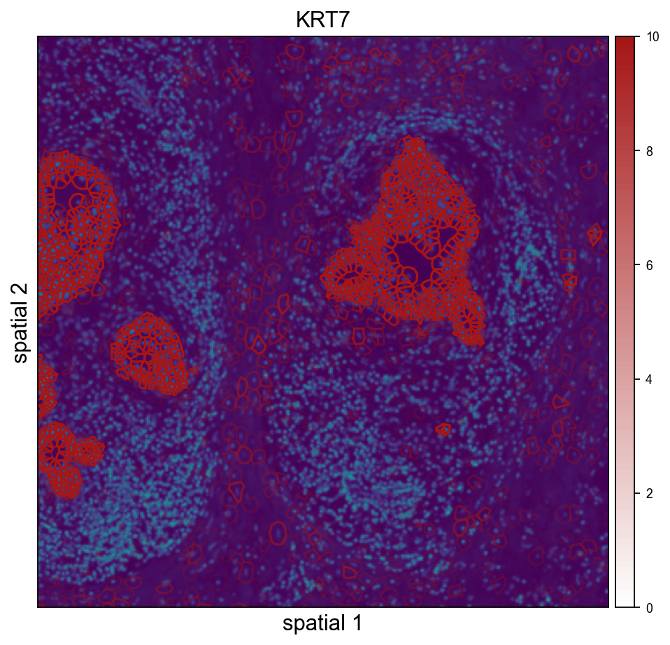
Cropped H&E / DAPI overlay — Leiden on the left, KRT7 on the right. crop_coord is in microns (same convention as the other spatialseg calls above); the loader’s rescaled tissue_hires_scalef handles the mapping into image-pixel space for the imshow call.

ov.pl.spatialseg(
    adata_img, color='leiden',
    library_id=library_id,
    edges_color='white', edges_width=0.4,
    # alpha=0.45 keeps the DAPI morphology visible through the cluster fills so the
    # polygon-to-nucleus alignment stays obvious. Raise closer to 1.0 if you only
    # care about cluster assignment and not the background.
    alpha=0.45, alpha_img=1.0,
    legend_fontsize=8,
    palette=ov.pl.palette_112,
    crop_coord=(2000, 3200, 2500, 3700),
    figsize=(7, 6),
)

<Axes: title={'center': 'leiden'}, xlabel='spatial 1', ylabel='spatial 2'>

ov.pl.spatialseg(
    adata_img, color=marker,
    library_id=library_id,
    edges_color='white', edges_width=0.4,
    alpha=0.65, alpha_img=1.0,
    legend_fontsize=8,
    cmap='Reds', vmax=vmax_marker,
    crop_coord=(2000, 3200, 2500, 3700),
    figsize=(7, 6),
)

<Axes: title={'center': 'KRT7'}, xlabel='spatial 1', ylabel='spatial 2'>

ov.pl.spatialseg(
    adata_img, color='KRT7',
    library_id=library_id,
    edges_color='white', edges_width=0.4,
    alpha=0.65, alpha_img=1.0,
    legend_fontsize=8,
    cmap=ov.pl.create_custom_colormap('#a51616'), vmax=10,
    crop_coord=(2000, 3200, 2500, 3700),
    figsize=(7, 6),
)

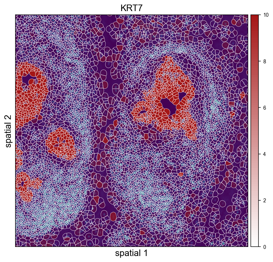
<Axes: title={'center': 'KRT7'}, xlabel='spatial 1', ylabel='spatial 2'>

ov.pl.spatialseg(
    adata_img, color='KRT7',
    library_id=library_id,
    edges_color='white', edges_width=0.4,
    alpha=0.65, alpha_img=1.0,
    legend_fontsize=8,
    cmap=ov.pl.create_custom_colormap('#a51616'), vmax=10,
    seg_contourpx=1.5,
    crop_coord=(2000, 3200, 2500, 3700),
    figsize=(7, 6),
)

<Axes: title={'center': 'KRT7'}, xlabel='spatial 1', ylabel='spatial 2'>

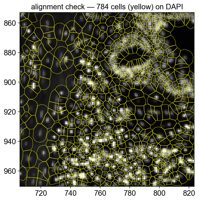
Quick alignment check — polygon outlines on DAPI

To confirm the morphology image and the cell polygons are correctly registered, render a tight crop with outlines only (no fill) over the DAPI background. Every polygon should contain exactly one DAPI-bright nucleus.

# Render polygons directly — gives full control of facecolor='none' so the fills
# don't mask the DAPI (`ov.pl.spatialseg(alpha=0, ...)` ends up skipping the
# collection entirely when alpha is zero).
import matplotlib.pyplot as plt
from matplotlib.patches import Polygon as _MplPoly
from matplotlib.collections import PatchCollection
from shapely import wkt as _wkt

x0u, x1u, y0u, y1u = 2400, 2800, 2900, 3300  # tighter crop (microns)
sf = adata_img.uns['spatial'][library_id]['scalefactors']['tissue_hires_scalef']
xy = adata_img.obsm['spatial']
mask = (xy[:,0] > x0u) & (xy[:,0] < x1u) & (xy[:,1] > y0u) & (xy[:,1] < y1u)

fig, ax = plt.subplots(figsize=(7, 6))
img = adata_img.uns['spatial'][library_id]['images']['hires']
ax.imshow(img, origin='upper', cmap='gray',
          vmax=float(np.percentile(img, 99.5)))
patches = []
for i in np.where(mask)[0]:
    w = adata_img.obs['geometry'].iloc[i]
    if not w: continue
    geom = _wkt.loads(w)
    if not hasattr(geom, 'exterior'): continue
    xs, ys = geom.exterior.xy
    pts = np.column_stack((np.array(xs)*sf, np.array(ys)*sf))
    patches.append(_MplPoly(pts, closed=True))
ax.add_collection(PatchCollection(
    patches, facecolor='none', edgecolor='yellow', linewidth=0.5, alpha=0.9,
))
ax.set_xlim(x0u * sf, x1u * sf)
ax.set_ylim(y1u * sf, y0u * sf)   # inverted y (image convention)
ax.set_title(f'alignment check — {len(patches)} cells (yellow) on DAPI')
ax.set_aspect('equal')
plt.show()