Real-data case study — MTBLS1 (urine NMR, Type 2 Diabetes)

The earlier notebooks use cachexia, synthetic drift data, or purpose-built factorial layouts. This one runs the full ov.metabol stack on a public, real-world dataset straight from the Metabolights repository: MTBLS1, a 600 MHz ¹H-NMR urine metabolomics study of Type 2 Diabetes (Salek et al., Physiol. Genomics 2007).

• 132 samples — 84 T2D, 48 controls

• 189 metabolite features (~30 % named, rest are chemical-shift peaks)

• No pooled-QC samples, no injection-order metadata → forces us to fall back on the non-QC code paths (cv_filter(across='all'))

• Pre-curated peak table in the study’s MAF file

Goals: (1) end-to-end workflow on data we did not generate; (2) show which tools apply and which don’t; (3) exercise every metabol plotting helper.

Workflow:

0. download the study

1. build an AnnData

2. QC & PCA-based sample outliers

3. missing-value pattern

4. intensity distribution (raw vs PQN-normalised)

5. impute / normalise / log+Pareto

6. two-group differential + volcano

7. PLS-DA, OPLS-DA, S-plot, VIP bar

8. MSEA ORA + pathway bar

9. ASCA (group × gender) + variance-explained bar

10. biomarker: per-feature ROC + nested-CV panel + fold ROC

11. DGCA + class-count bar + per-condition correlation network

12. summary

0 — Setup and dataset download

The whole ISA-Tab layout (sample sheet + assay sheet + MAF file) is fetched in one line with ov.utils.load_metabolights, which caches files under cache_dir and returns a samples × metabolites AnnData. group_col="Factor Value[Metabolic syndrome]" renames the T2D vs control factor to the canonical adata.obs['group'] so every downstream function works out of the box.

import numpy as np
import pandas as pd
import matplotlib.pyplot as plt
import omicverse as ov

ov.plot_set()
print('omicverse', ov.__version__)

🔬 Starting plot initialization...
🧬 Detecting GPU devices…
✅ NVIDIA CUDA GPUs detected: 1
    • [CUDA 0] NVIDIA H100 80GB HBM3
      Memory: 79.1 GB | Compute: 9.0

   ____            _     _    __                  
  / __ \____ ___  (_)___| |  / /__  _____________ 
 / / / / __ `__ \/ / ___/ | / / _ \/ ___/ ___/ _ \ 
/ /_/ / / / / / / / /__ | |/ /  __/ /  (__  )  __/ 
\____/_/ /_/ /_/_/\___/ |___/\___/_/  /____/\___/                                              

🔖 Version: 2.1.2rc1   📚 Tutorials: https://omicverse.readthedocs.io/
✅ plot_set complete.

omicverse 2.1.2rc1

adata = ov.utils.load_metabolights(
    'MTBLS1',
    group_col='Factor Value[Metabolic syndrome]',
    cache_dir='mtbls1_demo',
)
print(adata)
print('group counts:', adata.obs['group'].value_counts().to_dict())

AnnData object with n_obs × n_vars = 132 × 220
    obs: 'Source Name', 'Characteristics[Organism]', 'Term Source REF', 'Term Accession Number', 'Characteristics[Organism part]', 'Term Source REF.1', 'Term Accession Number.1', 'Characteristics[Variant]', 'Term Source REF.2', 'Term Accession Number.2', 'Characteristics[Sample type]', 'Term Source REF.3', 'Term Accession Number.3', 'Protocol REF', 'Factor Value[Gender]', 'Term Source REF.4', 'Term Accession Number.4', 'group', 'Term Source REF.5', 'Term Accession Number.5'
    var: 'metabolite_identification', 'chemical_formula', 'smiles'
    uns: 'metabolights'
group counts: {'Control Group': 84, 'diabetes mellitus': 48}

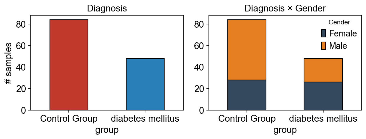
1 — Exploratory look

Before any cleaning, peek at the raw layout and gender breakdown so later per-step numbers are interpretable.

fig, axes = plt.subplots(1, 2, figsize=(8, 3.2))
adata.obs['group'].value_counts().plot.bar(ax=axes[0], color=['#c0392b', '#2980b9'], edgecolor='k')
axes[0].set_title('Diagnosis')
axes[0].set_ylabel('# samples')
axes[0].tick_params(axis='x', rotation=0)

pd.crosstab(adata.obs['group'], adata.obs['Factor Value[Gender]']).plot.bar(
    stacked=True, ax=axes[1], color=['#34495e', '#e67e22'], edgecolor='k')
axes[1].set_title('Diagnosis × Gender')
axes[1].legend(title='Gender', frameon=False)
axes[1].tick_params(axis='x', rotation=0)
fig.tight_layout(); plt.show()

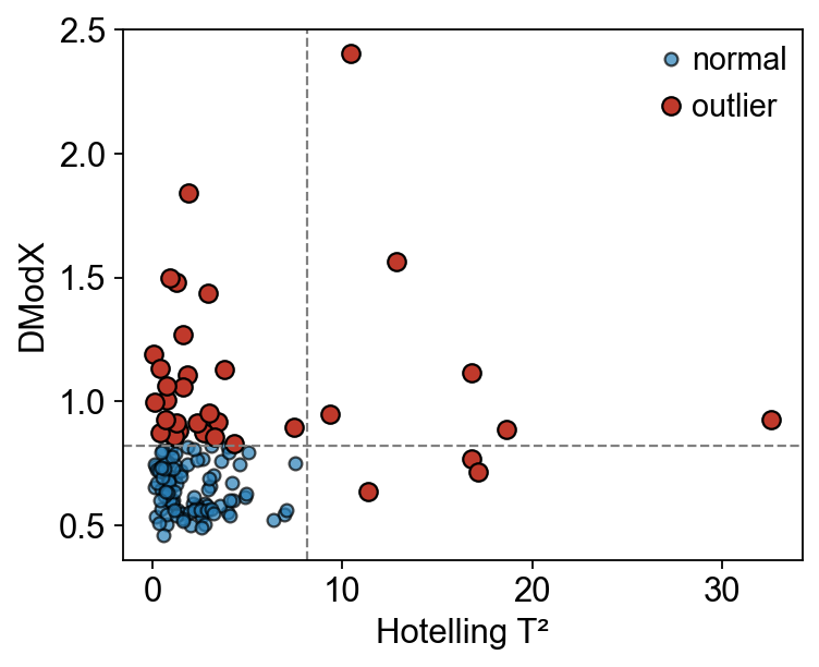
2 — Sample-level outlier detection (Hotelling T² + DModX)

sample_qc fits a PCA on the raw matrix, computes Hotelling’s T² (distance inside the PC-subspace) and DModX (distance to the residual plane), and flags samples that fall above either critical value at α = 0.95. sample_qc_plot renders the scatter + threshold lines in a single call.

qc = ov.metabol.sample_qc(adata, n_components=3, alpha=0.95)
print(f'flagged: {qc["is_outlier"].sum()} / {len(qc)}')
ov.metabol.sample_qc_plot(qc)
plt.show()

flagged: 35 / 132

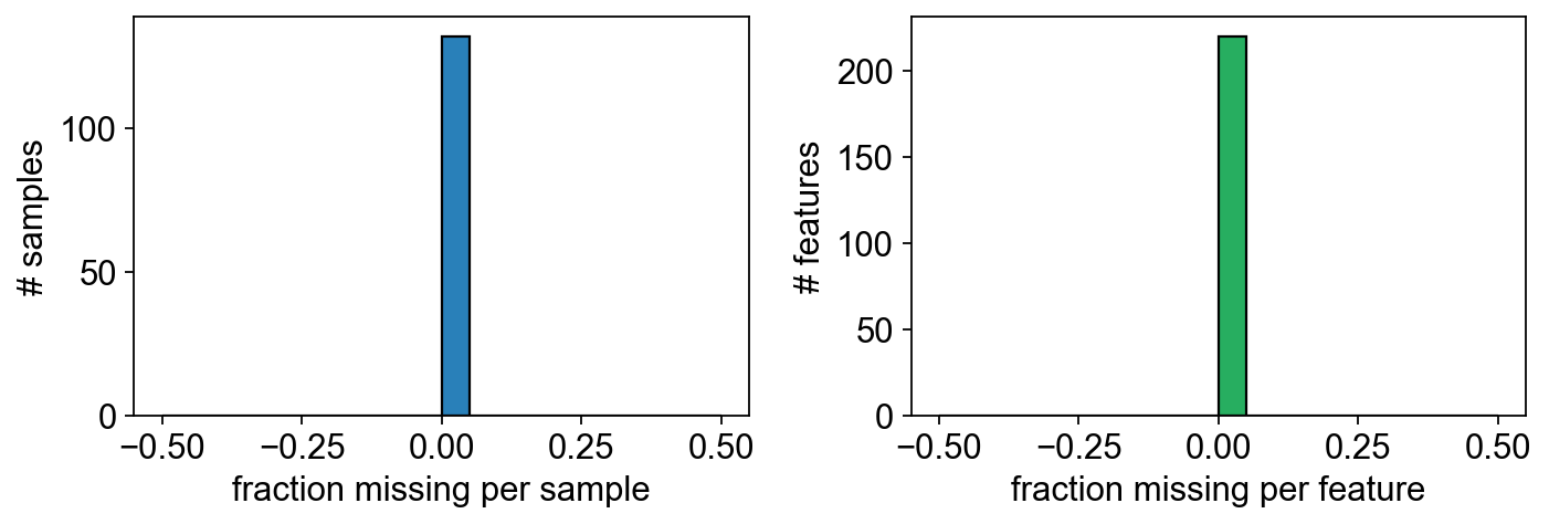
3 — Missing-value pattern

Before imputation, check where the NaNs sit. For a well-designed study the missing cells should be roughly uniform across samples — if one sample has 10× the NaN count of the others it probably needs dropping.

X = np.asarray(adata.X)
miss_per_sample = np.isnan(X).mean(axis=1)
miss_per_feature = np.isnan(X).mean(axis=0)
print(f'overall missingness: {np.isnan(X).mean():.1%}')
print(f'features with >10% NaN: {(miss_per_feature > 0.1).sum()}')

overall missingness: 0.0%
features with >10% NaN: 0

fig, axes = plt.subplots(1, 2, figsize=(9, 3.2))
axes[0].hist(miss_per_sample, bins=20, color='#2980b9', edgecolor='k')
axes[0].set_xlabel('fraction missing per sample'); axes[0].set_ylabel('# samples')
axes[1].hist(miss_per_feature, bins=20, color='#27ae60', edgecolor='k')
axes[1].set_xlabel('fraction missing per feature'); axes[1].set_ylabel('# features')
fig.tight_layout(); plt.show()

4 — Feature filter (cv_filter across=’all’) + preprocessing

cv_filter(across='all') is the v0.5 addition for QC-less studies: compute the CV across every sample (instead of pooled QC) and drop the noisiest features. Then impute with QRILC, normalise with PQN, log-transform, and Pareto-scale.

adata_cv = ov.metabol.cv_filter(adata, across='all', cv_threshold=1.5)
adata_imp = ov.metabol.impute(adata_cv, method='qrilc', seed=0)
adata_norm = ov.metabol.normalize(adata_imp, method='pqn')
adata_log = ov.metabol.transform(adata_norm, method='log')
adata_pareto = ov.metabol.transform(adata_log, method='pareto', stash_raw=False)

print(f'features kept by cv_filter: {adata_cv.n_vars}/{adata.n_vars}')
print(f'NaN after QRILC: {np.isnan(np.asarray(adata_imp.X)).sum()}')
print(f'Pareto max |column mean|: {np.abs(np.asarray(adata_pareto.X).mean(axis=0)).max():.2e}')

features kept by cv_filter: 194/220
NaN after QRILC: 0
Pareto max |column mean|: 3.32e-15

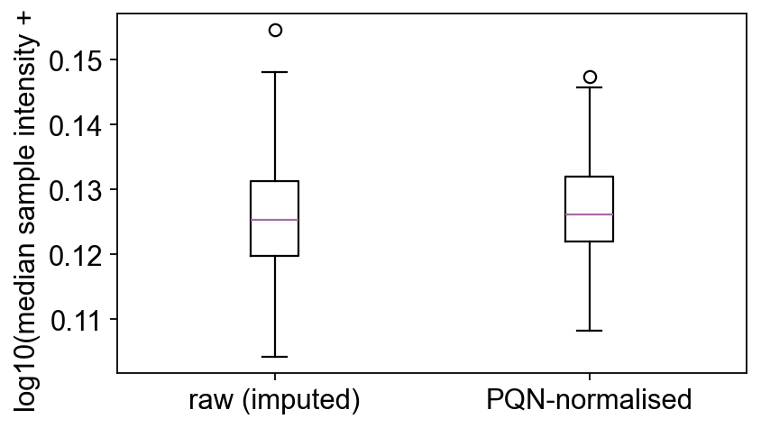
4a — Raw vs PQN-normalised intensity

A quick box-strip of per-sample median intensities before and after PQN — after normalisation all samples should sit at roughly the same level (the PQN assumption).

raw_med = np.log10(np.nanmedian(np.asarray(adata_imp.X), axis=1) + 1)
norm_med = np.log10(np.nanmedian(np.asarray(adata_norm.X), axis=1) + 1)
fig, ax = plt.subplots(figsize=(5.5, 3.2))
ax.boxplot([raw_med, norm_med], labels=['raw (imputed)', 'PQN-normalised'])
ax.set_ylabel('log10(median sample intensity + 1)')
fig.tight_layout(); plt.show()

5 — Two-group differential analysis (Welch’s t)

PQN + log is the MetaboAnalyst canonical pipeline; we ran it above. differential on the log-transformed AnnData gives per-feature Welch’s t, p-values, BH-FDR, and log2-fold changes.

deg = ov.metabol.differential(
    adata_log,
    group_col='group',
    group_a='diabetes mellitus',
    group_b='Control Group',
    method='welch_t',
    log_transformed=True,
)
print(f'{(deg["padj"] < 0.05).sum()}/{len(deg)} features padj<0.05')

78/194 features padj<0.05

top = deg.sort_values('pvalue').head(8).copy()
top['name'] = adata_cv.var.loc[top.index, 'metabolite_identification'].values
top[['name', 'stat', 'pvalue', 'padj', 'log2fc']]

                              name      stat        pvalue          padj  \
m59                     isoleucine -9.291729  4.663572e-16  4.523665e-14   
m60              N-acetylglutamate -9.291729  4.663572e-16  4.523665e-14   
m145  unknown_shift_[6.47 .. 6.52] -5.816492  4.601095e-08  2.975375e-06   
m195               unknown_m_8.335  5.716259  7.284739e-08  3.533098e-06   
m117          n-methylnicotinamide -5.551948  1.527003e-07  5.924770e-06   
m31                        ethanol  5.318509  1.895120e-06  5.252190e-05   
m30               2-oxoisovalerate  5.318509  1.895120e-06  5.252190e-05   
m184  unknown_shift_[7.81 .. 7.87] -5.022566  2.651056e-06  6.428810e-05   

        log2fc  
m59  -0.133335  
m60  -0.133335  
m145 -0.030824  
m195  0.043695  
m117 -0.223048  
m31   0.092268  
m30   0.092268  
m184 -0.498991  

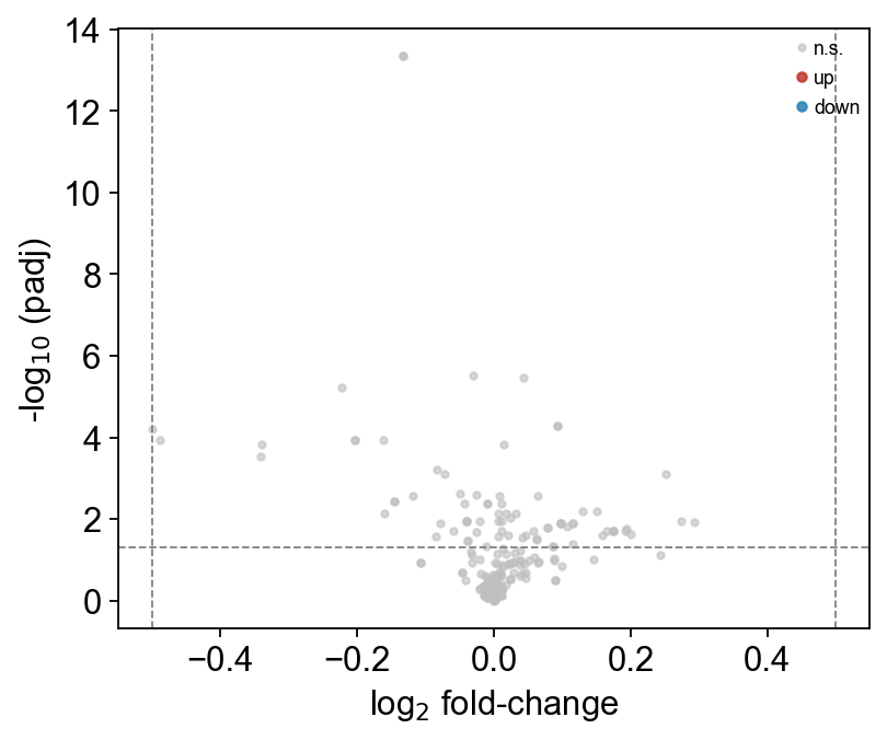
Volcano plot

ov.metabol.volcano(deg, padj_thresh=0.05, log2fc_thresh=0.5, label_top_n=8)
plt.show()

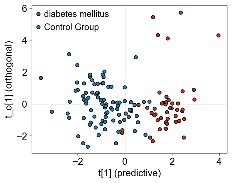
6 — Multivariate discrimination

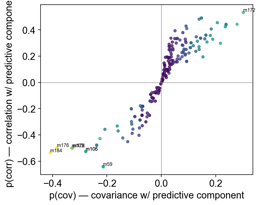
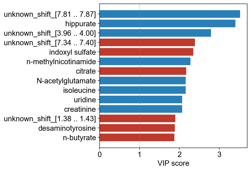
PLS-DA + OPLS-DA with leave-one-out Q² on the Pareto-scaled matrix. OPLS-DA adds the orthogonal-noise split that makes loadings interpretable; feed its result into s_plot (predictive-covariance vs correlation) and vip_bar for the Top-VIP ranking.

pls = ov.metabol.plsda(
    adata_pareto, group_col='group',
    group_a='diabetes mellitus', group_b='Control Group',
    n_components=2,
)
opls = ov.metabol.opls_da(
    adata_pareto, group_col='group',
    group_a='diabetes mellitus', group_b='Control Group',
    n_ortho=1,
)
print(f'PLS-DA  R²X={pls.r2x:.3f}  R²Y={pls.r2y:.3f}  Q²={pls.q2:.3f}')
print(f'OPLS-DA R²X={opls.r2x:.3f}  R²Y={opls.r2y:.3f}  Q²={opls.q2:.3f}')

PLS-DA  R²X=0.253  R²Y=0.669  Q²=0.566
OPLS-DA R²X=0.106  R²Y=0.669  Q²=0.566

OPLS-DA scores, S-plot, and VIP bar

fig, ax = plt.subplots(figsize=(5, 4))
for lbl, c in [('diabetes mellitus', '#c0392b'), ('Control Group', '#2980b9')]:
    mask = (adata_pareto.obs['group'] == lbl).to_numpy()
    ax.scatter(opls.scores[mask, 0], opls.x_ortho_scores[mask, 0], c=c, s=25,
               edgecolor='k', label=lbl)
ax.axvline(0, color='grey', lw=0.6); ax.axhline(0, color='grey', lw=0.6)
ax.set_xlabel('t[1] (predictive)'); ax.set_ylabel('t_o[1] (orthogonal)')
ax.legend(frameon=False); fig.tight_layout(); plt.show()

ov.metabol.s_plot(opls, adata_pareto, label_top_n=8)
plt.show()

# Use human-readable metabolite names on the VIP bars
mb_names = adata_pareto.var['metabolite_identification'].values
ov.metabol.vip_bar(opls, mb_names, top_n=15)
plt.show()

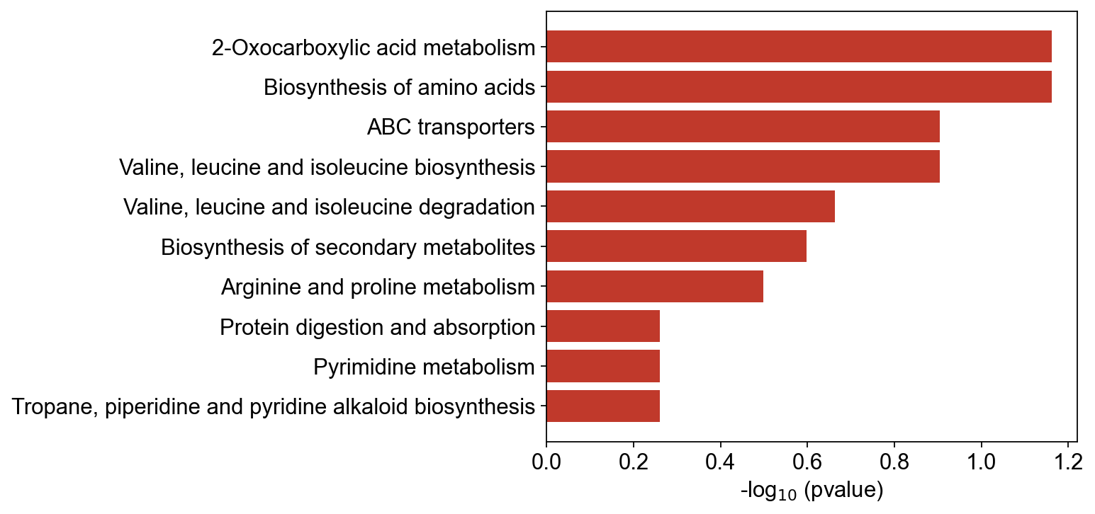
7 — Pathway enrichment (MSEA ORA)

MSEA resolves metabolite names → KEGG IDs. Passing mass_db= (v0.5 addition) makes the ChEBI table available as an in-memory lookup — names present there skip PubChem entirely. Combined with the cache-on-404 fix in fetch_hmdb_from_name, a warm cache run is about 100× faster than the cold one.

mass_db = ov.metabol.fetch_chebi_compounds()
hits = deg[deg['padj'] < 0.05].sort_values('padj').head(30).index.tolist()
hit_names = adata_cv.var.loc[hits, 'metabolite_identification'].tolist()
bg_names = adata_cv.var['metabolite_identification'].dropna().tolist()
enr = ov.metabol.msea_ora(hit_names, bg_names, mass_db=mass_db)
print(f'{len(enr)} pathways tested, {(enr["padj"] < 0.05).sum()} padj<0.05')
enr.sort_values('padj').head(5)[['pathway', 'overlap', 'set_size', 'odds_ratio', 'padj']]

18 pathways tested, 0 padj<0.05

                                       pathway  overlap  set_size  odds_ratio  \
0              2-Oxocarboxylic acid metabolism        3         5    6.857143   
1                  Biosynthesis of amino acids        3         5    6.857143   
2                             ABC transporters        2         3    8.250000   
3  Valine, leucine and isoleucine biosynthesis        2         3    8.250000   
4   Valine, leucine and isoleucine degradation        2         4    4.000000   

       padj  
0  0.560631  
1  0.560631  
2  0.560631  
3  0.560631  
4  0.658375  

ov.metabol.pathway_bar(enr, top_n=10)
plt.show()

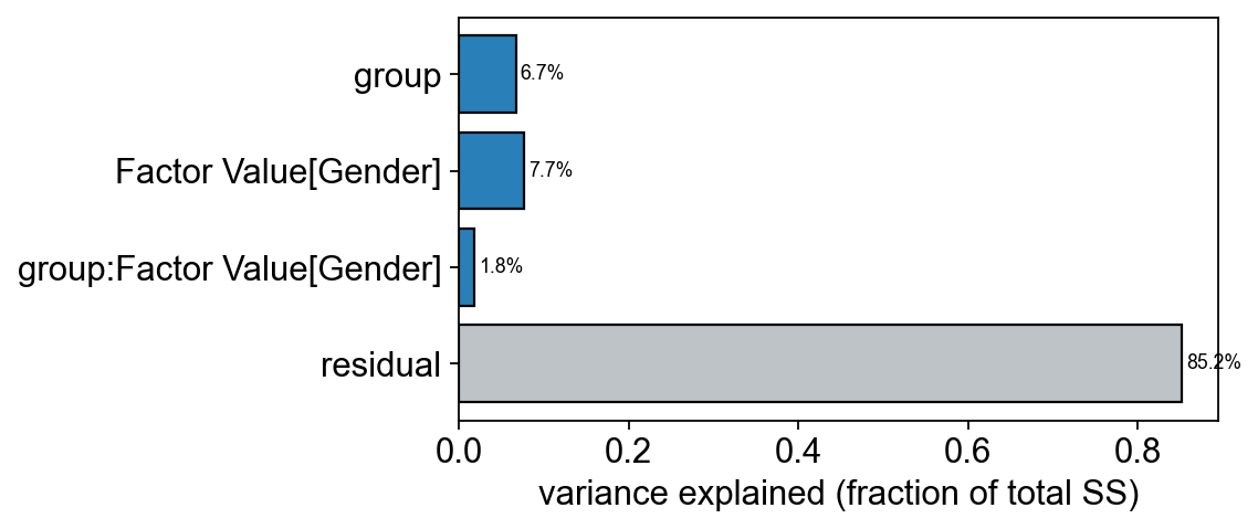
8 — Multi-factor decomposition (ASCA)

ASCA decomposes the centred data into per-factor effect matrices plus interactions plus residual. On MTBLS1 we have group (T2D vs control) and gender — and ASCA quantifies how much variance each explains globally.

asca = ov.metabol.asca(
    adata_pareto,
    factors=['group', 'Factor Value[Gender]'],
    include_interactions=True,
    n_permutations=100,
    seed=0,
)
asca.summary().round(4)

                       effect         ss   df  variance_explained  p_value
0                       group   204.6645  1.0              0.0670   0.0099
1        Factor Value[Gender]   235.3499  1.0              0.0770   0.0099
2  group:Factor Value[Gender]    56.1278  1.0              0.0184   0.0198
3                    residual  2602.8727  NaN              0.8519      NaN

ov.metabol.asca_variance_bar(asca)
plt.show()

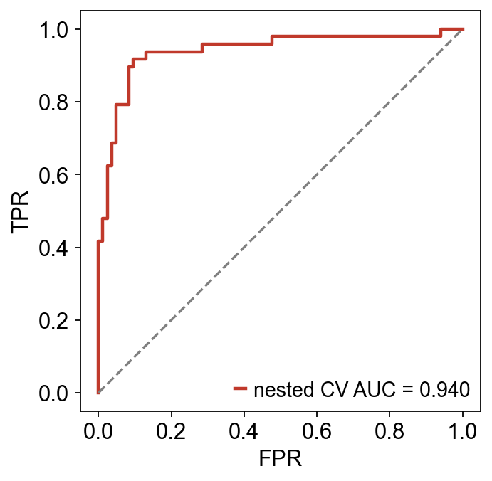
9 — Biomarker discovery: per-feature ROC + nested-CV panel

roc_feature gives polarity-invariant per-feature AUC. biomarker_panel runs a multivariate nested CV (5-outer × 3-inner L2 logistic regression here) on the top-10 features with a 100- permutation null.

auc = ov.metabol.roc_feature(
    adata_log, group_col='group',
    pos_group='diabetes mellitus', neg_group='Control Group',
)
top_auc = auc.head(10).copy()
top_auc['name'] = adata_cv.var.loc[top_auc.index, 'metabolite_identification'].values
top_auc[['name', 'auc']]

                              name       auc
m60              N-acetylglutamate  0.901166
m59                     isoleucine  0.901166
m30               2-oxoisovalerate  0.815972
m31                        ethanol  0.815972
m184  unknown_shift_[7.81 .. 7.87]  0.766369
m117          n-methylnicotinamide  0.758681
m176                     hippurate  0.758185
m178                     hippurate  0.757192
m103  unknown_shift_[3.96 .. 4.00]  0.748760
m127  unknown_shift_[5.33 .. 5.36]  0.743056

fig, ax = plt.subplots(figsize=(5, 3.2))
ax.hist(auc['auc'], bins=20, color='#2980b9', edgecolor='k')
ax.axvline(0.7, color='#c0392b', ls='--', label='AUC = 0.7')
ax.set_xlabel('per-feature AUC'); ax.set_ylabel('# metabolites')
ax.legend(frameon=False); fig.tight_layout(); plt.show()
print(f'{(auc["auc"] >= 0.7).sum()} metabolites with AUC ≥ 0.7')

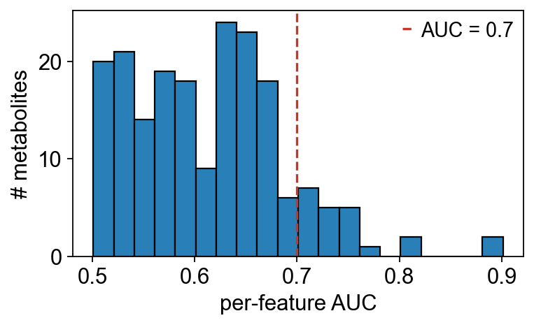
22 metabolites with AUC ≥ 0.7

panel = ov.metabol.biomarker_panel(
    adata_log, group_col='group',
    pos_group='diabetes mellitus', neg_group='Control Group',
    features=10, classifier='lr',
    cv_outer=5, cv_inner=3, n_permutations=100, seed=0,
)
print(f'nested CV AUC: {panel.mean_auc:.3f} ± {panel.std_auc:.3f}')
print(f'permutation p-value: {panel.permutation_pvalue:.3f}')

nested CV AUC: 0.946 ± 0.037
permutation p-value: 0.010

from sklearn.metrics import roc_curve, auc as _auc
fpr, tpr, _ = roc_curve(panel.outer_labels, panel.outer_predictions)
fig, ax = plt.subplots(figsize=(4.5, 4.5))
ax.plot(fpr, tpr, color='#c0392b', lw=2, label=f'nested CV AUC = {_auc(fpr, tpr):.3f}')
ax.plot([0, 1], [0, 1], ls='--', color='grey')
ax.set_xlabel('FPR'); ax.set_ylabel('TPR'); ax.set_aspect('equal')
ax.legend(loc='lower right'); fig.tight_layout(); plt.show()

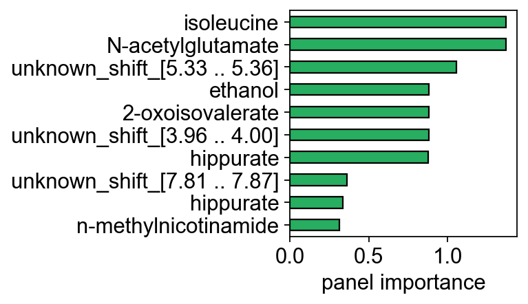
fig, ax = plt.subplots(figsize=(5, 3))
imp = panel.feature_importance
imp.index = adata_cv.var.loc[imp.index, 'metabolite_identification'].values
imp.iloc[::-1].plot.barh(ax=ax, color='#27ae60', edgecolor='k')
ax.set_xlabel('panel importance'); ax.set_ylabel('')
fig.tight_layout(); plt.show()

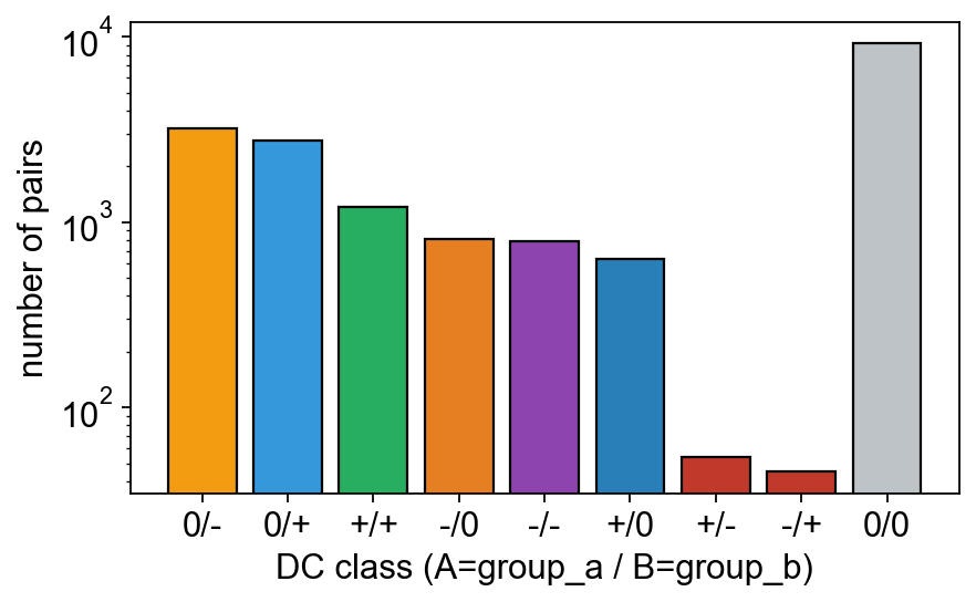
10 — Differential correlation (DGCA) + static network

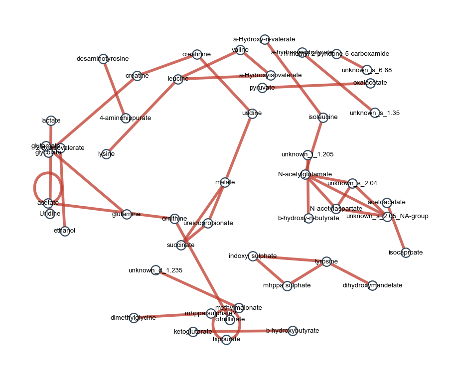
DGCA classifies every metabolite-pair correlation as one of +/+ -/- +/- -/+ +/0 0/+ -/0 0/- 0/0. The class-count bar shows the overall rewiring landscape; the corr_network network plot on the T2D condition reveals the backbone that survives the |r| ≥ 0.5 filter.

dc = ov.metabol.dgca(
    adata_log, group_col='group',
    group_a='diabetes mellitus', group_b='Control Group',
    method='spearman',
)
print(f'{len(dc)} pairs, {(dc["padj"] < 0.05).sum()} padj<0.05')
dc.sort_values('padj').head(5)[['feature_a', 'feature_b', 'r_a', 'r_b', 'z_diff', 'padj']]

18721 pairs, 2887 padj<0.05

   feature_a feature_b       r_a       r_b     z_diff      padj
0       m149      m150  1.000000  0.999656  40.478362  0.000000
1       m148      m218 -0.212657  0.749357  -6.386681  0.000002
8        m51       m59 -0.029744  0.784732  -5.848193  0.000006
10       m68      m198  0.207013 -0.709142   5.892204  0.000006
14      m148      m210 -0.111919  0.762155  -5.990206  0.000006

ov.metabol.dgca_class_bar(dc)
plt.show()

edges_t2d = ov.metabol.corr_network(
    adata_log,
    group_col='group', group='diabetes mellitus',
    method='spearman',
    abs_r_threshold=0.5, padj_threshold=0.05,
)
print(f'{len(edges_t2d)} edges in T2D network (|r|≥0.5, padj<0.05)')

740 edges in T2D network (|r|≥0.5, padj<0.05)

named = adata_cv.var['metabolite_identification'].to_dict()
edges_plot = edges_t2d.copy()
edges_plot['feature_a'] = edges_plot['feature_a'].map(named).fillna(edges_plot['feature_a'])
edges_plot['feature_b'] = edges_plot['feature_b'].map(named).fillna(edges_plot['feature_b'])
top = edges_plot.head(40)
ov.metabol.corr_network_plot(top, figsize=(7, 6), label_font_size=6)
plt.show()

11 — Pipeline summary

Step	Status on MTBLS1	Plot shown
ov.utils.load_metabolights	✓	—
exploratory bar chart	✓	1 (group × gender)
cv_filter(across='all')	✓	—
sample_qc + sample_qc_plot	✓	1 (T² vs DModX)
missing-value histograms	✓	1 (two panels)
raw vs PQN box	✓	1
impute / normalize / transform	✓	—
differential + volcano	✓	1 (volcano)
plsda / opls_da / s_plot / vip_bar	✓	3
msea_ora(mass_db=) + pathway_bar	✓	1
asca + asca_variance_bar	✓	1
roc_feature + AUC histogram	✓	1
biomarker_panel + fold ROC + feature-importance bar	✓	2
dgca + dgca_class_bar	✓	1
corr_network + corr_network_plot	✓	1
drift_correct, serrf	✗ (no QC pool)	—
mixed_model, meba	✗ (cross-sectional)	—
run_mofa	✗ (mono-omic)	—

~15 plots across the pipeline. Every plot cell uses one visualization helper from ov.metabol.* (or a 3-line matplotlib snippet for the one-off summaries) so each cell stays under five callable references.