k-means — the trivial baseline that’s often hard to beat#
sklearn’s standard k-means; no metacell-specific paper.
Algorithm. Run k-means on the PCA embedding; each cluster is one metacell. Cluster centroid = “codebook” entry.
Capabilities. latent, codebook, out_of_sample.
Strengths. Trivial to implement. Free out-of-sample projection via
predict. Cluster centroids are interpretable. No new dependencies beyond
sklearn.
Weaknesses. No notion of cell-cell graph; metacell boundaries are straight-line Voronoi cuts in PCA space, which may not respect manifold structure. No soft assignments.
This is the “honest first thing to try” baseline. If kmeans is within
a few percent of seacells on your purity / DE benchmarks, you may not
need the heavier methods.
1. Setup#
# Standard imports + omicverse defaults.
import warnings
warnings.filterwarnings('ignore')

import numpy as np
import pandas as pd
import omicverse as ov
import scvelo as scv      # only used for the demo dataset

ov.plot_set()
🔬 Starting plot initialization...
🧬 Detecting GPU devices…
✅ NVIDIA CUDA GPUs detected: 1
    • [CUDA 0] NVIDIA H100 80GB HBM3
      Memory: 79.1 GB | Compute: 9.0

   ____            _     _    __
  / __ \____ ___  (_)___| |  / /__  _____________
 / / / / __ `__ \/ / ___/ | / / _ \/ ___/ ___/ _ \
/ /_/ / / / / / / / /__ | |/ /  __/ /  (__  )  __/
\____/_/ /_/ /_/_/\___/ |___/\___/_/  /____/\___/

🔖 Version: 2.2.0   📚 Tutorials: https://omicverse.readthedocs.io/
✅ plot_set complete.
2. Load and preprocess#
# Pancreas scRNA-seq (Bastidas-Ponce et al. 2019). Standard omicverse
# preprocess flow: qc -> preprocess -> scale -> pca -> neighbors -> umap.
adata = scv.datasets.pancreas()
adata = ov.pp.qc(adata,
                 tresh={'mito_perc': 0.20, 'nUMIs': 500, 'detected_genes': 250},
                 mt_startswith='mt-')
adata = ov.pp.preprocess(adata, mode='shiftlog|pearson', n_HVGs=2000)
adata.layers['lognorm'] = adata.X.copy()        # mcRigor reads this
adata = adata[:, adata.var.highly_variable_features]
ov.pp.scale(adata)
ov.pp.pca(adata, layer='scaled', n_pcs=30)
adata.obsm['X_pca'] = adata.obsm['scaled|original|X_pca']
ov.pp.neighbors(adata, n_neighbors=15, use_rep='X_pca')
ov.pp.umap(adata)
print('adata:', adata.shape, 'celltypes:', sorted(adata.obs['clusters'].unique()))
🖥️ Using CPU mode for QC...

📊 Step 1: Calculating QC Metrics

   ✓ Gene Family Detection:
   ┌──────────────────────────────┬────────────────────┬────────────────────┐
   │ Gene Family                  │ Genes Found        │ Detection Method   │
   ├──────────────────────────────┼────────────────────┼────────────────────┤
   │ Mitochondrial                │ 13                 │ Auto (MT-)         │
   ├──────────────────────────────┼────────────────────┼────────────────────┤
   │ Ribosomal                    │ 0 ⚠️               │ Auto (RPS/RPL)     │
   ├──────────────────────────────┼────────────────────┼────────────────────┤
   │ Hemoglobin                   │ 0 ⚠️               │ Auto (regex)       │
   └──────────────────────────────┴────────────────────┴────────────────────┘

   ✓ QC Metrics Summary:
   ┌─────────────────────────┬────────────────────┬─────────────────────────┐
   │ Metric                  │ Mean               │ Range (Min - Max)       │
   ├─────────────────────────┼────────────────────┼─────────────────────────┤
   │ nUMIs                   │ 6675               │ 3020 - 18524            │
   ├─────────────────────────┼────────────────────┼─────────────────────────┤
   │ Detected Genes          │ 2516               │ 1473 - 4492             │
   ├─────────────────────────┼────────────────────┼─────────────────────────┤
   │ Mitochondrial %         │ 0.7%               │ 0.2% - 4.3%             │
   ├─────────────────────────┼────────────────────┼─────────────────────────┤
   │ Ribosomal %             │ 0.0%               │ 0.0% - 0.0%             │
   ├─────────────────────────┼────────────────────┼─────────────────────────┤
   │ Hemoglobin %            │ 0.0%               │ 0.0% - 0.0%             │
   └─────────────────────────┴────────────────────┴─────────────────────────┘

   📈 Original cell count: 3,696

🔧 Step 2: Quality Filtering (SEURAT)
   Thresholds: mito≤0.2, nUMIs≥500, genes≥250
   📊 Seurat Filter Results:
     • nUMIs filter (≥500): 0 cells failed (0.0%)
     • Genes filter (≥250): 0 cells failed (0.0%)
     • Mitochondrial filter (≤0.2): 0 cells failed (0.0%)
   ✓ Filters applied successfully
   ✓ Combined QC filters: 0 cells removed (0.0%)

🎯 Step 3: Final Filtering
   Parameters: min_genes=200, min_cells=3
   Ratios: max_genes_ratio=1, max_cells_ratio=1
✓ Final filtering: 0 cells, 12,261 genes removed

🔍 Step 4: Doublet Detection
   💡 Running pyscdblfinder (Python port of R scDblFinder)
   🔍 Running scdblfinder detection...
[ScDblFinder] wrote scDblFinder_score + scDblFinder_class — threshold=0.387
   ✓ scDblFinder completed: 66 doublets removed (1.8%)

╭─ SUMMARY: qc ──────────────────────────────────────────────────────╮
│  Duration: 17.3602s                                                │
│  Shape:    3,696 x 27,998 (Unchanged)                              │
│                                                                    │
│  CHANGES DETECTED                                                  │
│  ────────────────                                                  │
│  ● OBS    │ ✚ cell_complexity (float)                              │
│           │ ✚ detected_genes (int)                                 │
│           │ ✚ hb_perc (float)                                      │
│           │ ✚ mito_perc (float)                                    │
│           │ ✚ nUMIs (float)                                        │
│           │ ✚ n_counts (float)                                     │
│           │ ✚ n_genes (int)                                        │
│           │ ✚ n_genes_by_counts (int)                              │
│           │ ✚ passing_mt (bool)                                    │
│           │ ✚ passing_nUMIs (bool)                                 │
│           │ ✚ passing_ngenes (bool)                                │
│           │ ✚ pct_counts_hb (float)                                │
│           │ ✚ pct_counts_mt (float)                                │
│           │ ✚ pct_counts_ribo (float)                              │
│           │ ✚ ribo_perc (float)                                    │
│           │ ✚ total_counts (float)                                 │
│                                                                    │
│  ● VAR    │ ✚ hb (bool)                                            │
│           │ ✚ mt (bool)                                            │
│           │ ✚ ribo (bool)                                          │
│                                                                    │
╰────────────────────────────────────────────────────────────────────╯
🔍 [2026-05-19 17:23:55] Running preprocessing in 'cpu' mode...
Begin robust gene identification
    After filtration, 15737/15737 genes are kept.
    Among 15737 genes, 15736 genes are robust.
✅ Robust gene identification completed successfully.
Begin size normalization: shiftlog and HVGs selection pearson
🔍 Count Normalization:
   Target sum: 500000.0
   Exclude highly expressed: True
   Max fraction threshold: 0.2
   ⚠️ Excluding 1 highly-expressed genes from normalization computation
   Excluded genes: ['Ghrl']
✅ Count Normalization Completed Successfully!
   ✓ Processed: 3,630 cells × 15,736 genes
   ✓ Runtime: 0.25s

🔍 Highly Variable Genes Selection (Experimental):
   Method: pearson_residuals
   Target genes: 2,000
   Theta (overdispersion): 100
✅ Experimental HVG Selection Completed Successfully!
   ✓ Selected: 2,000 highly variable genes out of 15,736 total (12.7%)
   ✓ Results added to AnnData object:
     • 'highly_variable': Boolean vector (adata.var)
     • 'highly_variable_rank': Float vector (adata.var)
     • 'highly_variable_nbatches': Int vector (adata.var)
     • 'highly_variable_intersection': Boolean vector (adata.var)
     • 'means': Float vector (adata.var)
     • 'variances': Float vector (adata.var)
     • 'residual_variances': Float vector (adata.var)
    Time to analyze data in cpu: 1.51 seconds.
✅ Preprocessing completed successfully.
    Added:
        'highly_variable_features', boolean vector (adata.var)
        'means', float vector (adata.var)
        'variances', float vector (adata.var)
        'residual_variances', float vector (adata.var)
        'counts', raw counts layer (adata.layers)
    End of size normalization: shiftlog and HVGs selection pearson

╭─ SUMMARY: preprocess ──────────────────────────────────────────────╮
│  Duration: 1.8978s                                                 │
│  Shape:    3,630 x 15,737 -> 3,630 x 15,736                        │
│                                                                    │
│  CHANGES DETECTED                                                  │
│  ────────────────                                                  │
│  ● VAR    │ ✚ highly_variable (bool)                               │
│           │ ✚ highly_variable_features (bool)                      │
│           │ ✚ highly_variable_rank (float)                         │
│           │ ✚ means (float)                                        │
│           │ ✚ n_cells (int)                                        │
│           │ ✚ percent_cells (float)                                │
│           │ ✚ residual_variances (float)                           │
│           │ ✚ robust (bool)                                        │
│           │ ✚ variances (float)                                    │
│                                                                    │
│  ● UNS    │ ✚ history_log                                          │
│           │ ✚ hvg                                                  │
│           │ ✚ log1p                                                │
│                                                                    │
│  ● LAYERS │ ✚ counts (sparse matrix, 3630x15736)                   │
│                                                                    │
╰────────────────────────────────────────────────────────────────────╯
╭─ SUMMARY: scale ───────────────────────────────────────────────────╮
│  Duration: 0.6758s                                                 │
│  Shape:    3,630 x 2,000 (Unchanged)                               │
│                                                                    │
│  CHANGES DETECTED                                                  │
│  ────────────────                                                  │
│  ● LAYERS │ ✚ scaled (array, 3630x2000)                            │
│                                                                    │
╰────────────────────────────────────────────────────────────────────╯
computing PCA🔍
    with n_comps=30
   🖥️ Using sklearn PCA for CPU computation
   🖥️ sklearn PCA backend: CPU computation
   📊 PCA input data type: ArrayView, shape: (3630, 2000), dtype: float64
🔧 PCA solver used: covariance_eigh
    finished✅ (1.64s)

╭─ SUMMARY: pca ─────────────────────────────────────────────────────╮
│  Duration: 1.6465s                                                 │
│  Shape:    3,630 x 2,000 (Unchanged)                               │
│                                                                    │
│  CHANGES DETECTED                                                  │
│  ────────────────                                                  │
│  ● UNS    │ ✚ scaled|original|cum_sum_eigenvalues                  │
│           │ ✚ scaled|original|pca_var_ratios                       │
│                                                                    │
│  ● OBSM   │ ✚ scaled|original|X_pca (array, 3630x30)               │
│                                                                    │
╰────────────────────────────────────────────────────────────────────╯
🖥️ Using Scanpy CPU to calculate neighbors...

🔍 K-Nearest Neighbors Graph Construction:
   Mode: cpu
   Neighbors: 15
   Method: umap
   Metric: euclidean
   Representation: X_pca
   🔍 Computing neighbor distances...
🔍 Computing connectivity matrix...
   💡 Using UMAP-style connectivity
✓ Graph is fully connected

✅ KNN Graph Construction Completed Successfully!
   ✓ Processed: 3,630 cells with 15 neighbors each
   ✓ Results added to AnnData object:
     • 'neighbors': Neighbors metadata (adata.uns)
     • 'distances': Distance matrix (adata.obsp)
     • 'connectivities': Connectivity matrix (adata.obsp)

╭─ SUMMARY: neighbors ───────────────────────────────────────────────╮
│  Duration: 8.6927s                                                 │
│  Shape:    3,630 x 2,000 (Unchanged)                               │
│                                                                    │
│  CHANGES DETECTED                                                  │
│  ────────────────                                                  │
╰────────────────────────────────────────────────────────────────────╯
🔍 [2026-05-19 17:24:08] Running UMAP in 'cpu' mode...
🖥️ Using Scanpy CPU UMAP...

🔍 UMAP Dimensionality Reduction:
   Mode: cpu
   Method: umap
   Components: 2
   Min distance: 0.5
{'n_neighbors': 15, 'method': 'umap', 'random_state': 0, 'metric': 'euclidean', 'use_rep': 'X_pca'}
   🔍 Computing UMAP parameters...
   🔍 Computing UMAP embedding (classic method)...
✅ UMAP Dimensionality Reduction Completed Successfully!
   ✓ Embedding shape: 3,630 cells × 2 dimensions
   ✓ Results added to AnnData object:
     • 'X_umap': UMAP coordinates (adata.obsm)
     • 'umap': UMAP parameters (adata.uns)
✅ UMAP completed successfully.

╭─ SUMMARY: umap ────────────────────────────────────────────────────╮
│  Duration: 0.8348s                                                 │
│  Shape:    3,630 x 2,000 (Unchanged)                               │
│                                                                    │
│  CHANGES DETECTED                                                  │
│  ────────────────                                                  │
│  ● UNS    │ ✚ umap                                                 │
│           │ └─ params: {'a': 0.5830300199950147, 'b': 1.334166993228519}│
│                                                                    │
╰────────────────────────────────────────────────────────────────────╯
adata: (3630, 2000) celltypes: ['Alpha', 'Beta', 'Delta', 'Ductal', 'Epsilon', 'Ngn3 high EP', 'Ngn3 low EP', 'Pre-endocrine']
3. Fit k-means#
sklearn k-means; n_init=10 runs 10 random initialisations and picks the
best (by inertia).
mc = ov.single.MetaCell(
    adata.copy(), method='kmeans', n_metacells=100,
    use_rep='X_pca', n_init=10, random_state=0,
).fit()
print(f'inertia: {mc._fit_result.backend_meta["inertia"]:.0f}')
inertia: 235416
4. AnnData schema after fit#
Every backend writes the same fields into adata — that’s what lets the
downstream helpers below work without branching on the backend.
# Inspect what the fit wrote into adata via the unified schema.
print(f'method      : {mc.method}')
print(f'capabilities: {sorted(mc.capabilities)}')
print(f'n_metacells : {np.unique(mc._fit_result.assignments).size}')
print(f'runtime     : {mc._fit_result.runtime_s:.3f} s')
print(f'uns         : {dict(mc.adata.uns["metacell"])}')
method      : kmeans
capabilities: ['codebook', 'latent', 'out_of_sample']
n_metacells : 100
runtime     : 5.011 s
uns         : {'method': 'kmeans', 'n_metacells': 100, 'n_iter': 35, 'converged': True, 'runtime_s': 5.011103391647339, 'random_state': 0, 'capabilities': ['codebook', 'latent', 'out_of_sample']}
5. Aggregate to a metacell AnnData#
predicted(method='hard', layer='counts', summary='sum') returns a
metacell × gene AnnData with raw count totals preserved — the format that
downstream tools (SCENIC, CellPhoneDB, pseudobulk DE) actually want.
ad_mc = mc.predicted(method='hard', layer='counts', summary='sum',
                     celltype_label='clusters')
print(f'metacell AnnData: {ad_mc.shape}')
print(f'mean cells/metacell: {ad_mc.obs["n_cells"].mean():.1f}')
ad_mc.obs.head()
metacell AnnData: (100, 2000)
mean cells/metacell: 36.3
| n_cells | clusters | clusters_purity | |
|---|---|---|---|
| mc-0 | 58 | Ductal | 0.879310 |
| mc-1 | 25 | Pre-endocrine | 0.760000 |
| mc-2 | 39 | Ngn3 high EP | 1.000000 |
| mc-3 | 31 | Beta | 1.000000 |
| mc-4 | 37 | Alpha | 0.972973 |
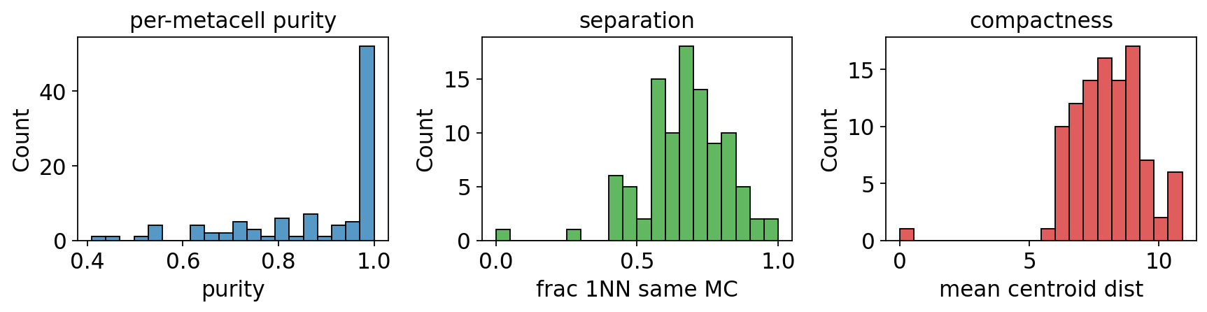
6. Benchmarking metrics (purity / separation / compactness)#
# Compute purity / separation / compactness AND show the 3-panel histogram
# in one call (ov.pl.metacell_metrics returns the per-metacell tables too).
purity, separation, compactness = ov.pl.metacell_metrics(
    mc, label_key='clusters', use_rep='X_pca',
)
7. mcRigor: statistical validation#
For each metacell, mcRigor permutes the (cells × genes) submatrix in two
ways and asks: is the observed gene–gene covariance bigger than the null
distribution at this metacell’s size? Metacells whose mcDiv exceeds the
size-stratified threshold are flagged as 'dubious'.
# mcRigor's double-permutation null. dubious_rate = fraction of cells in
# heterogeneous metacells; rigor_score = 1 - 0.5*(dubious_rate + zero_rate).
rep = mc.check_rigor(layer_lognorm='lognorm', n_rep=20,
                     feature_use=1000, random_state=0)
print(f'rigor_score : {rep.score:.3f}')
print(f'dubious_rate: {rep.dubious_rate:.3f}')
print(f'zero_rate   : {rep.zero_rate:.3f}')
print(f'# metacells : {rep.n_metacells}')
rigor_score : 0.673
dubious_rate: 0.411
zero_rate   : 0.244
# metacells : 100
7.1 Per-metacell mcDiv vs size#
# mcDiv vs metacell size, overlaid with size-stratified threshold.
ov.pl.rigor_scatter(rep)
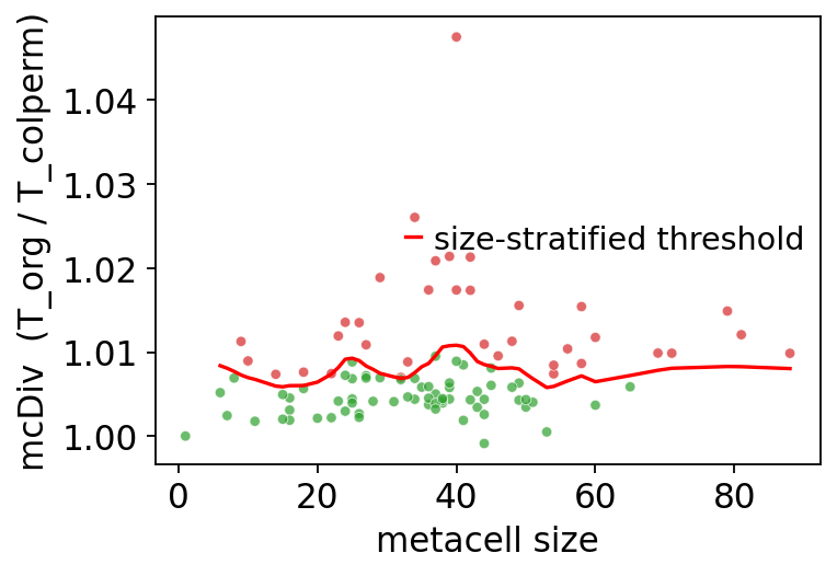
<Axes: xlabel='metacell size', ylabel='mcDiv (T_org / T_colperm)'>
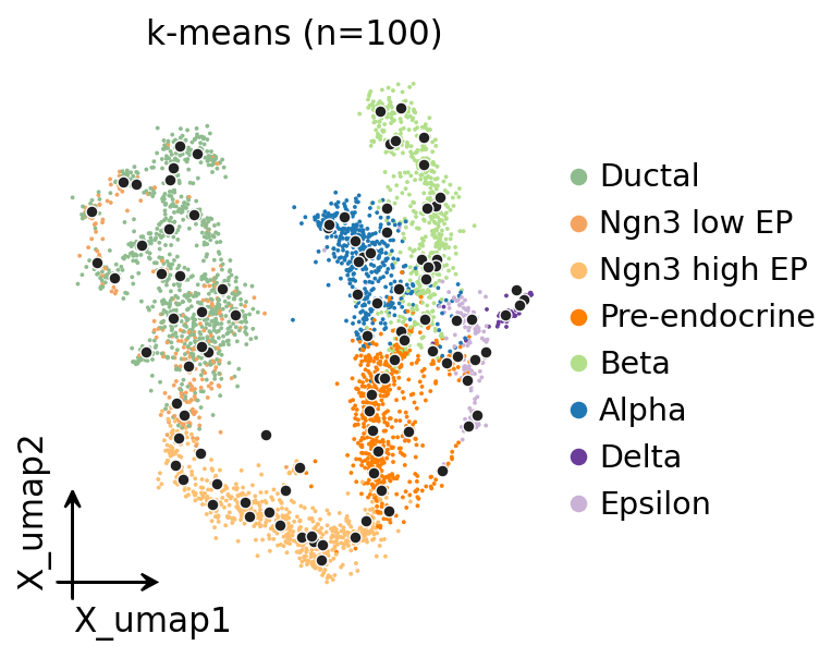
8. UMAP with metacell centroids#
# UMAP coloured by celltype with metacell centroids overlaid in dark grey.
import matplotlib.pyplot as plt
fig, ax = plt.subplots(figsize=(5, 4))
ov.pl.embedding(mc.adata, basis='X_umap', color='clusters', ax=ax, show=False,
                frameon='small', title='k-means (n=100)', size=12)
labels = mc._fit_result.assignments
pts = np.array([mc.adata.obsm['X_umap'][labels == u].mean(axis=0)
                for u in np.unique(labels)])
ax.scatter(pts[:, 0], pts[:, 1], s=24, c='#222',
           edgecolors='white', linewidths=0.6, zorder=5)
plt.tight_layout(); plt.show()
9. Per-celltype purity boxplot#
# Per-celltype boxplot of metacell purity.
ov.pl.metacell_purity_box(mc, label_key='clusters')
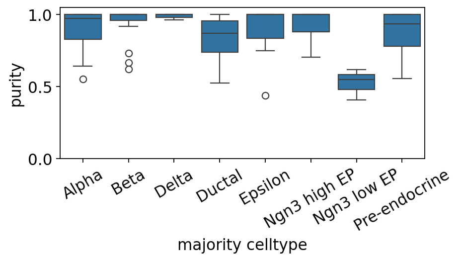
<Axes: xlabel='majority celltype', ylabel='purity'>
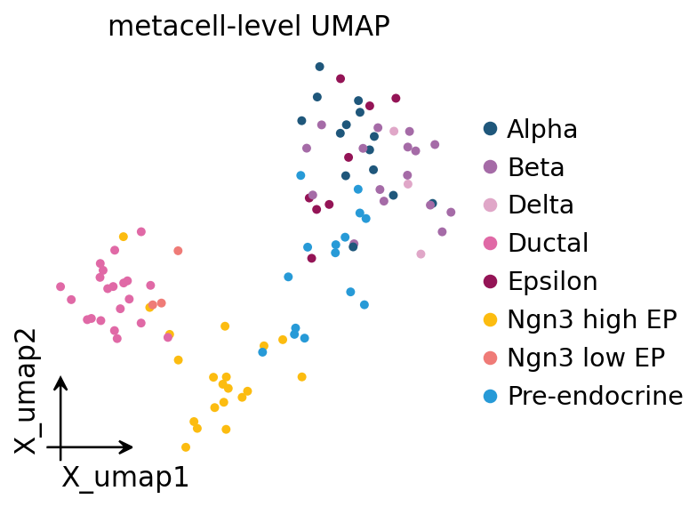
10. Metacell-level UMAP#
A common downstream use of metacells is to treat them as a much smaller “atlas” of pseudo-cells and re-run the standard omicverse preprocess → PCA → UMAP loop on them. Cell-type signal should survive.
# Treat the metacell AnnData as a smaller dataset and run the standard
# omicverse preprocess -> pca -> neighbors -> umap loop on it.
ad_mc = ov.pp.preprocess(ad_mc, mode='shiftlog|pearson',
                          n_HVGs=min(2000, ad_mc.n_vars))
ad_mc = ad_mc[:, ad_mc.var.highly_variable_features]
ov.pp.scale(ad_mc)
ov.pp.pca(ad_mc, layer='scaled', n_pcs=min(30, ad_mc.n_obs - 1))
ad_mc.obsm['X_pca'] = ad_mc.obsm['scaled|original|X_pca']
ov.pp.neighbors(ad_mc, n_neighbors=min(15, ad_mc.n_obs - 1), use_rep='X_pca')
ov.pp.umap(ad_mc)
ov.pl.embedding(ad_mc, basis='X_umap', color='clusters',
                frameon='small', title='metacell-level UMAP', size=80)
🔍 [2026-05-19 17:24:45] Running preprocessing in 'cpu' mode...
Begin robust gene identification
    After filtration, 2000/2000 genes are kept.
    Among 2000 genes, 2000 genes are robust.
✅ Robust gene identification completed successfully.
Begin size normalization: shiftlog and HVGs selection pearson

🔍 Count Normalization:
   Target sum: 500000.0
   Exclude highly expressed: True
   Max fraction threshold: 0.2
   ⚠️ Excluding 1 highly-expressed genes from normalization computation
   Excluded genes: ['Ghrl']

✅ Count Normalization Completed Successfully!
   ✓ Processed: 100 cells × 2,000 genes
   ✓ Runtime: 0.00s

🔍 Highly Variable Genes Selection (Experimental):
   Method: pearson_residuals
   Target genes: 2,000
   Theta (overdispersion): 100

✅ Experimental HVG Selection Completed Successfully!
   ✓ Selected: 2,000 highly variable genes out of 2,000 total (100.0%)
   ✓ Results added to AnnData object:
     • 'highly_variable': Boolean vector (adata.var)
     • 'highly_variable_rank': Float vector (adata.var)
     • 'highly_variable_nbatches': Int vector (adata.var)
     • 'highly_variable_intersection': Boolean vector (adata.var)
     • 'means': Float vector (adata.var)
     • 'variances': Float vector (adata.var)
     • 'residual_variances': Float vector (adata.var)
    Time to analyze data in cpu: 0.03 seconds.
✅ Preprocessing completed successfully.
    Added:
        'highly_variable_features', boolean vector (adata.var)
        'means', float vector (adata.var)
        'variances', float vector (adata.var)
        'residual_variances', float vector (adata.var)
        'counts', raw counts layer (adata.layers)
    End of size normalization: shiftlog and HVGs selection pearson

╭─ SUMMARY: preprocess ──────────────────────────────────────────────╮
│  Duration: 0.0444s                                                 │
│  Shape:    100 x 2,000 (Unchanged)                                 │
│                                                                    │
│  CHANGES DETECTED                                                  │
│  ────────────────                                                  │
│  ● UNS    │ ✚ REFERENCE_MANU                                       │
│           │ ✚ _ov_provenance                                       │
│           │ ✚ history_log                                          │
│           │ ✚ hvg                                                  │
│           │ ✚ log1p                                                │
│           │ ✚ status                                               │
│           │ ✚ status_args                                          │
│                                                                    │
│  ● LAYERS │ ✚ counts (sparse matrix, 100x2000)                     │
│                                                                    │
╰────────────────────────────────────────────────────────────────────╯

╭─ SUMMARY: scale ───────────────────────────────────────────────────╮
│  Duration: 0.0137s                                                 │
│  Shape:    100 x 2,000 (Unchanged)                                 │
│                                                                    │
│  CHANGES DETECTED                                                  │
│  ────────────────                                                  │
│  ● LAYERS │ ✚ scaled (array, 100x2000)                             │
│                                                                    │
╰────────────────────────────────────────────────────────────────────╯
computing PCA🔍
    with n_comps=30
   🖥️ Using sklearn PCA for CPU computation
   🖥️ sklearn PCA backend: CPU computation
   📊 PCA input data type: ArrayView, shape: (100, 2000), dtype: float64
🔧 PCA solver used: covariance_eigh
    finished✅ (0.98s)

╭─ SUMMARY: pca ─────────────────────────────────────────────────────╮
│  Duration: 0.9824s                                                 │
│  Shape:    100 x 2,000 (Unchanged)                                 │
│                                                                    │
│  CHANGES DETECTED                                                  │
│  ────────────────                                                  │
│  ● UNS    │ ✚ pca                                                  │
│           │ └─ params: {'zero_center': True, 'use_highly_variable': Tr...│
│           │ ✚ scaled|original|cum_sum_eigenvalues                  │
│           │ ✚ scaled|original|pca_var_ratios                       │
│                                                                    │
│  ● OBSM   │ ✚ X_pca (array, 100x30)                                │
│           │ ✚ scaled|original|X_pca (array, 100x30)                │
│                                                                    │
╰────────────────────────────────────────────────────────────────────╯
🖥️ Using Scanpy CPU to calculate neighbors...

🔍 K-Nearest Neighbors Graph Construction:
   Mode: cpu
   Neighbors: 15
   Method: umap
   Metric: euclidean
   Representation: X_pca
   🔍 Computing neighbor distances...
   🔍 Computing connectivity matrix...
   💡 Using UMAP-style connectivity
   ✓ Graph is fully connected

✅ KNN Graph Construction Completed Successfully!
   ✓ Processed: 100 cells with 15 neighbors each
   ✓ Results added to AnnData object:
     • 'neighbors': Neighbors metadata (adata.uns)
     • 'distances': Distance matrix (adata.obsp)
     • 'connectivities': Connectivity matrix (adata.obsp)

╭─ SUMMARY: neighbors ───────────────────────────────────────────────╮
│  Duration: 0.1064s                                                 │
│  Shape:    100 x 2,000 (Unchanged)                                 │
│                                                                    │
│  CHANGES DETECTED                                                  │
│  ────────────────                                                  │
│  ● UNS    │ ✚ neighbors                                            │
│           │ └─ params: {'n_neighbors': 15, 'method': 'umap', 'random_s...│
│                                                                    │
│  ● OBSP   │ ✚ connectivities (sparse matrix, 100x100)              │
│           │ ✚ distances (sparse matrix, 100x100)                   │
│                                                                    │
╰────────────────────────────────────────────────────────────────────╯
🔍 [2026-05-19 17:24:46] Running UMAP in 'cpu' mode...
🖥️ Using Scanpy CPU UMAP...

🔍 UMAP Dimensionality Reduction:
   Mode: cpu
   Method: umap
   Components: 2
   Min distance: 0.5
{'n_neighbors': 15, 'method': 'umap', 'random_state': 0, 'metric': 'euclidean', 'use_rep': 'X_pca'}
   🔍 Computing UMAP parameters...
   🔍 Computing UMAP embedding (classic method)...

✅ UMAP Dimensionality Reduction Completed Successfully!
   ✓ Embedding shape: 100 cells × 2 dimensions
   ✓ Results added to AnnData object:
     • 'X_umap': UMAP coordinates (adata.obsm)
     • 'umap': UMAP parameters (adata.uns)
✅ UMAP completed successfully.

╭─ SUMMARY: umap ────────────────────────────────────────────────────╮
│  Duration: 0.0116s                                                 │
│  Shape:    100 x 2,000 (Unchanged)                                 │
│                                                                    │
│  CHANGES DETECTED                                                  │
│  ────────────────                                                  │
│  ● UNS    │ ✚ umap                                                 │
│           │ └─ params: {'a': 0.5830300199950147, 'b': 1.334166993228519}│
│                                                                    │
│  ● OBSM   │ ✚ X_umap (array, 100x2)                                │
│                                                                    │
╰────────────────────────────────────────────────────────────────────╯
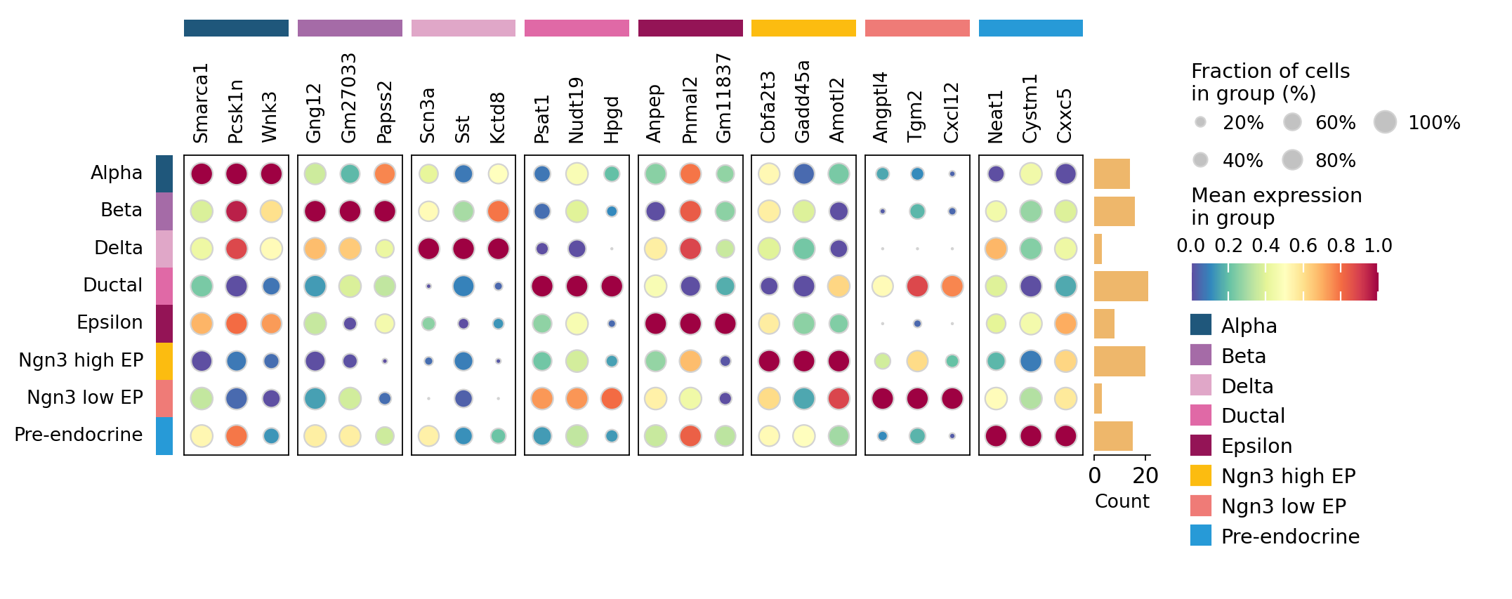
11. Top markers per celltype on the metacell AnnData#
# Find top markers per celltype on the metacell AnnData (omicverse helper —
# drops the categories with <2 metacells automatically and reports cell-type
# fractions ``pts`` along with the gene names).
counts = ad_mc.obs['clusters'].value_counts()
keep = counts[counts >= 2].index.tolist()
ad_mc_for_de = ad_mc[ad_mc.obs['clusters'].isin(keep)].copy()
ad_mc_for_de.obs['clusters'] = ad_mc_for_de.obs['clusters'].astype('category')

ov.single.find_markers(ad_mc_for_de, groupby='clusters', method='wilcoxon',
                       key_added='rank_genes_groups', pts=True, use_gpu=False)
ov.single.get_markers(ad_mc_for_de, n_genes=3, key='rank_genes_groups')
🔍 Finding marker genes | method: wilcoxon | groupby: clusters | n_groups: 8 | n_genes: 50
✅ Done | 8 groups × 50 genes | corr: benjamini-hochberg | stored in adata.uns['rank_genes_groups']
| group | rank | names | scores | logfoldchanges | pvals | pvals_adj | pct_group | pct_rest | |
|---|---|---|---|---|---|---|---|---|---|
| 0 | Alpha | 1 | Smarca1 | 5.761621 | 3.176778 | 8.330991e-09 | 1.183973e-05 | 1.0 | 0.976744 |
| 1 | Alpha | 2 | Pcsk1n | 5.702018 | 4.696618 | 1.183973e-08 | 1.183973e-05 | 1.0 | 0.965116 |
| 2 | Alpha | 3 | Wnk3 | 5.612614 | 4.574257 | 1.992933e-08 | 1.328622e-05 | 1.0 | 0.697674 |
| 3 | Beta | 1 | Gng12 | 6.280682 | 4.077652 | 3.370923e-10 | 1.447338e-07 | 1.0 | 0.952381 |
| 4 | Beta | 2 | Gm27033 | 6.261877 | 4.418585 | 3.803710e-10 | 1.447338e-07 | 1.0 | 0.761905 |
| 5 | Beta | 3 | Papss2 | 6.252475 | 5.376971 | 4.039991e-10 | 1.447338e-07 | 1.0 | 0.619048 |
| 6 | Delta | 1 | Scn3a | 2.939994 | 5.103552 | 3.282187e-03 | 2.016374e-01 | 1.0 | 0.443299 |
| 7 | Delta | 2 | Sst | 2.939994 | 12.304194 | 3.282187e-03 | 2.016374e-01 | 1.0 | 0.752577 |
| 8 | Delta | 3 | Kctd8 | 2.939994 | 5.570514 | 3.282187e-03 | 2.016374e-01 | 1.0 | 0.412371 |
| 9 | Ductal | 1 | Psat1 | 7.019774 | 5.464606 | 2.222273e-12 | 3.414306e-10 | 1.0 | 0.670886 |
| 10 | Ductal | 2 | Nudt19 | 7.011312 | 3.159677 | 2.360946e-12 | 3.414306e-10 | 1.0 | 0.987342 |
| 11 | Ductal | 3 | Hpgd | 7.002849 | 6.883746 | 2.508096e-12 | 3.414306e-10 | 1.0 | 0.329114 |
| 12 | Epsilon | 1 | Anpep | 4.675616 | 4.504535 | 2.930724e-06 | 6.929630e-04 | 1.0 | 0.934783 |
| 13 | Epsilon | 2 | Pnmal2 | 4.675616 | 2.209542 | 2.930724e-06 | 6.929630e-04 | 1.0 | 0.956522 |
| 14 | Epsilon | 3 | Gm11837 | 4.675616 | 6.127854 | 2.930724e-06 | 6.929630e-04 | 1.0 | 0.641304 |
| 15 | Ngn3 high EP | 1 | Cbfa2t3 | 6.859351 | 3.967570 | 6.917419e-12 | 2.024575e-09 | 1.0 | 0.862500 |
| 16 | Ngn3 high EP | 2 | Gadd45a | 6.850733 | 5.042740 | 7.347228e-12 | 2.024575e-09 | 1.0 | 0.987500 |
| 17 | Ngn3 high EP | 3 | Amotl2 | 6.807647 | 4.025137 | 9.920783e-12 | 2.024575e-09 | 1.0 | 0.875000 |
| 18 | Ngn3 low EP | 1 | Angptl4 | 2.939994 | 4.896341 | 3.282187e-03 | 2.075064e-01 | 1.0 | 0.391753 |
| 19 | Ngn3 low EP | 2 | Tgm2 | 2.899582 | 4.878219 | 3.736610e-03 | 2.075064e-01 | 1.0 | 0.628866 |
| 20 | Ngn3 low EP | 3 | Cxcl12 | 2.859169 | 5.561907 | 4.247519e-03 | 2.075064e-01 | 1.0 | 0.329897 |
| 21 | Pre-endocrine | 1 | Neat1 | 5.902980 | 2.777033 | 3.569938e-09 | 2.729572e-06 | 1.0 | 0.788235 |
| 22 | Pre-endocrine | 2 | Cystm1 | 5.845060 | 1.281761 | 5.063850e-09 | 2.729572e-06 | 1.0 | 1.000000 |
| 23 | Pre-endocrine | 3 | Cxxc5 | 5.738874 | 1.267457 | 9.530800e-09 | 2.729572e-06 | 1.0 | 0.988235 |
# Dotplot of top markers per metacell-level celltype.
ov.pl.markers_dotplot(ad_mc_for_de, groupby='clusters', n_genes=3,
                      key='rank_genes_groups')
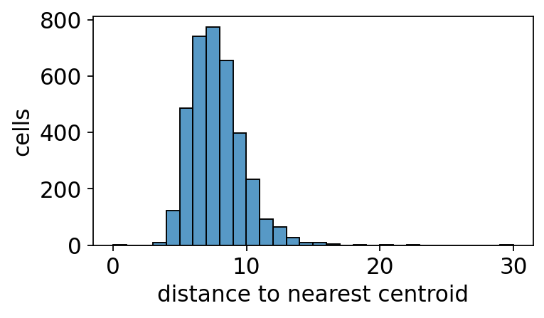
12. k-means exclusive: out-of-sample projection via cluster centroids#
Free out-of-sample projection — every new cell snaps to its nearest centroid in PCA space. No re-fit needed. Also lets us inspect the per-cell distance to the assigned centroid as a confidence proxy.
# Same out-of-sample API as MetaQ.
new_cells = adata[:500].copy()
assign = mc.assign_new_cells(new_cells)
for k, v in assign.items():
    print(f'  {k:12s}: shape={v.shape}, dtype={v.dtype}')
print(f'\nmean confidence (1/(1+distance)): {assign["confidence"].mean():.3f}')
metacell_id : shape=(500,), dtype=int64
  confidence  : shape=(500,), dtype=float32
  embedding   : shape=(500, 30), dtype=float32

mean confidence (1/(1+distance)): 0.118
# Per-cell distance to assigned centroid → confidence proxy.
import seaborn as sns
import matplotlib.pyplot as plt
X = mc.adata.obsm['X_pca']
labels = mc._fit_result.assignments
centroids = mc.codebook()
per_cell_d = np.linalg.norm(X - centroids[labels], axis=1)
print(f'distance to centroid (X_pca):')
print(f'  mean : {per_cell_d.mean():.3f}, median: {np.median(per_cell_d):.3f}, '
      f'max: {per_cell_d.max():.3f}')

fig, ax = plt.subplots(figsize=(5, 3))
sns.histplot(per_cell_d, bins=30, ax=ax, color='#1f77b4')
ax.set_xlabel('distance to nearest centroid'); ax.set_ylabel('cells')
plt.tight_layout(); plt.show()
distance to centroid (X_pca):
  mean : 7.805, median: 7.565, max: 29.976
13. Save / load roundtrip#
# Save/load roundtrip — every backend supports this.
import tempfile, os
with tempfile.NamedTemporaryFile(suffix='.pkl', delete=False) as f:
    path = f.name
mc.save(path)

mc2 = ov.single.MetaCell(adata.copy(), method='kmeans', n_metacells=100,
                          use_rep='X_pca', random_state=0)
mc2.load(path)
print(f'saved+loaded {path}')
os.remove(path)
saved+loaded /tmp/tmpabwwu73d.pkl
14. Takeaways#
k-means in PCA space is fast, simple, and surprisingly competitive on purity in many published benchmarks.
Use it as your first sanity check. If
kmeansalready givesmean_purity > 0.8anddubious_rate < 0.05, the more expensive methods may not be worth the runtime.Limitation: Voronoi cuts in PCA space can split a curved manifold at the “wrong” place; SEACells / MetaQ are kinder to manifolds.