Metabolomics preprocessing and univariate statistics

Metabolomics preprocessing and univariate statistics#

This is the first tutorial in the omicverse metabolomics series. It walks through the downstream analysis of a peak-intensity table — the matrix you get out of XCMS / MZmine / MS-DIAL / MetaboAnalyst — and builds up every step of the canonical statistical workflow with explicit rationale for each methodological choice.

By the end you will understand:

What an AnnData object looks like for metabolomics and why it’s the right container
The two kinds of “missing” in LC-MS data (MAR vs MNAR) and which imputer matches which
Why PQN (Dieterle 2006) is the de-facto standard sample normalization and not TIC
Why Pareto scaling (not z-score) is used before OPLS-DA
How BH-FDR interacts with small-n metabolomics studies

Dataset: Eisner et al. 2010 urine NMR cachexia study — 77 samples (47 cachexic cancer patients + 30 healthy controls), 63 NMR-quantified metabolites. One of the canonical MetaboAnalyst demo datasets.

Other tutorials in this series:

t_metabol_02_multivariate.ipynb — PLS-DA / OPLS-DA / VIP / S-plot
t_metabol_03_pathway.ipynb — ID mapping + MSEA (ORA + GSEA)
t_metabol_04_untargeted.ipynb — LC-MS peak lists + mummichog (real malaria dataset)
t_metabol_05_lipidomics.ipynb — LIPID MAPS parsing + LION enrichment (real breast-cancer dataset)

0 — Setup#

We only import omicverse — every metabolomics function is accessed through ov.metabol.* so the notebook stays terse and users can discover the API via tab-completion on ov.metabol.

import matplotlib.pyplot as plt
import numpy as np

import omicverse as ov

ov.plot_set()
print('omicverse', ov.__version__)

🔬 Starting plot initialization...
🧬 Detecting GPU devices…
✅ NVIDIA CUDA GPUs detected: 1
    • [CUDA 0] NVIDIA H100 80GB HBM3
      Memory: 79.1 GB | Compute: 9.0

   ____            _     _    __                  
  / __ \____ ___  (_)___| |  / /__  _____________ 
 / / / / __ `__ \/ / ___/ | / / _ \/ ___/ ___/ _ \ 
/ /_/ / / / / / / / /__ | |/ /  __/ /  (__  )  __/ 
\____/_/ /_/ /_/_/\___/ |___/\___/_/  /____/\___/                                              

🔖 Version: 2.1.2rc1   📚 Tutorials: https://omicverse.readthedocs.io/
✅ plot_set complete.

omicverse 2.1.2rc1

1 — Download the dataset#

ov.datasets.download_data(url, file_path, dir) is omicverse’s robust downloader — it has a progress bar, automatic parent-directory creation, and is idempotent (if the file already exists it won’t re-download). Use this rather than urllib.request, which has no progress, no retry, and puts the file in whatever working directory the notebook happens to be in.

The cachexia CSV is hosted by MetaboAnalyst at their public REST mirror; it’s ~32 KB.

csv_path = ov.datasets.download_data(
    url='https://rest.xialab.ca/api/download/metaboanalyst/human_cachexia.csv',
    file_path='human_cachexia.csv',
    dir='./metabol_data',
)
print('local path:', csv_path)

🔍 Downloading data to ./metabol_data/human_cachexia.csv
✅ Download completed
local path: ./metabol_data/human_cachexia.csv

2 — Load the peak table into AnnData#

ov.metabol.read_metaboanalyst is the right reader for the MetaboAnalyst bulk-upload CSV format, which MetaboAnalyst documents here:

Rows are samples. Column 1 is a sample ID. Column 2 is the grouping factor. Columns 3… are metabolite concentrations, one per column.

The reader’s three important arguments:

Argument	Meaning	Default
`path`	CSV path or URL	required
`group_col`	Name of the factor column (varies by dataset)	`"Muscle loss"` (matches the cachexia demo)
`sample_col`	Name of the sample-ID column	`None` → the first column

The return is an AnnData — the standard container for omicverse, also for scanpy / squidpy / monocle2_py / miloR_py. Samples become rows of adata.X, metabolites become columns. This makes every omicverse preprocessing / plotting utility work on metabolomics data out-of-the-box.

adata = ov.metabol.read_metaboanalyst(csv_path, group_col='Muscle loss')
print(adata)
print('\ngroup split:', adata.obs['group'].value_counts().to_dict())
print('\nfirst 5 metabolites:', list(adata.var_names[:5]))
print('raw intensity range: {:.2f} .. {:.2f}'.format(adata.X.min(), adata.X.max()))

AnnData object with n_obs × n_vars = 77 × 63
    obs: 'group'

group split: {'cachexic': 47, 'control': 30}

first 5 metabolites: ['1,6-Anhydro-beta-D-glucose', '1-Methylnicotinamide', '2-Aminobutyrate', '2-Hydroxyisobutyrate', '2-Oxoglutarate']
raw intensity range: 0.79 .. 33860.35

The raw intensity range (0.79 .. 33860) is two orders of magnitude — a classic symptom that variance-stabilizing transform is required before any parametric statistics.

3 — Missing values: why imputer choice matters#

In LC-MS and NMR there are two fundamentally different reasons a metabolite can be missing in a sample:

Type	Cause	Right imputer
MAR (missing-at-random)	technical dropout — ion suppression, poor peak picking, matrix effect	kNN (fill from similar samples)
MNAR (missing-not-at-random)	concentration below detection limit	QRILC / half-min (draw from the left tail)

Blindly using kNN on MNAR dropouts inflates false positives downstream because it fills low-abundance holes with mid-range values from “similar” samples; using half-min on MAR dropouts is overly pessimistic. A reasonable default for untargeted LC-MS is QRILC — it estimates the left-tail mean/sd from the lowest-q% of each feature’s observed values and draws from a truncated normal there, giving sensible MNAR imputations.

The cachexia NMR data has no missing values, so imputation is a no-op here. We spike in 10% random NaNs purely to demonstrate the API and compare the four imputers’ behavior on known truth.

rng = np.random.default_rng(0)
adata_hole = adata.copy()
mask = rng.random(adata_hole.X.shape) < 0.10
X = adata_hole.X.astype(float).copy()
X[mask] = np.nan
adata_hole.X = X
print(f'spiked NaN fraction: {np.isnan(adata_hole.X).mean():.3f}')

# Compare imputers on the same synthetic hole pattern
for method in ('zero', 'half_min', 'knn', 'qrilc'):
    imp = ov.metabol.impute(adata_hole, method=method,
                            missing_threshold=0.5,
                            n_neighbors=5,
                            q=0.01)
    # Compare imputed values to the true values we deleted
    err = np.nanmean((imp.X[mask] - adata.X[mask]) ** 2) ** 0.5
    print(f'  {method:10s}  n_vars_kept={imp.n_vars:3d}  RMSE vs truth = {err:.3f}')

spiked NaN fraction: 0.105
  zero        n_vars_kept= 63  RMSE vs truth = 1461.034
  half_min    n_vars_kept= 63  RMSE vs truth = 1403.251
  knn         n_vars_kept= 63  RMSE vs truth = 663.290
  qrilc       n_vars_kept= 63  RMSE vs truth = 1378.835

On this clean-ish dataset the kNN imputer wins on RMSE — which makes sense: the “missingness” we injected is synthetic MAR (completely random), exactly the regime kNN is designed for. On real LC-MS data where roughly half the missingness is MNAR, QRILC usually ties or beats kNN. Report which imputer you used in your paper.

For the rest of the tutorial we work with the original, unperturbed cachexia data.

4 — Sample normalization (PQN)#

Every sample in an LC-MS / NMR experiment has a slightly different total amount of material — different extraction efficiency, different injection volume, different NMR probe tuning. Sample normalization removes this dilution effect so samples become comparable.

Why PQN and not TIC#

Method	Divides each sample by…	When to use
TIC (total ion current)	sample sum	Simple but assumes total metabolite load is biologically irrelevant — rarely true
median	sample median	Robust to a few high outlier features but still wastes information
MSTUS	sum of stable features only	TIC with an outlier filter
PQN	sample median of ratios to a reference spectrum	Corrects dilution without assuming anything about total load

PQN (Dieterle et al. 2006, Anal Chem) is the community default for metabolomics. The intuition: pick a reference spectrum (element-wise median of all samples), divide each sample by it feature-by-feature, then the median of those ratios per sample is the dilution factor to remove. Since it uses the median, a handful of biologically-changed metabolites don’t throw off the scale.

ov.metabol.normalize parameters:

Parameter	Meaning	Default
`method`	`"pqn"`, `"tic"`, `"median"`, `"mstus"`	`"pqn"`
`reference`	only for PQN — `"median"` (robust) or `"mean"`	`"median"` (matches MetaboAnalyst)
`missing_threshold`	only for MSTUS — exclude features missing in > this fraction from the denominator	0.5

normed = ov.metabol.normalize(adata, method='pqn')

# QC: dispersion of row medians should tighten after PQN (samples more comparable)
raw_row_med = np.median(adata.X, axis=1)
pqn_row_med = np.median(normed.X, axis=1)
print(f'row-median dispersion (max/min) — raw: {raw_row_med.max()/raw_row_med.min():.2f}'
      f'   PQN: {pqn_row_med.max()/pqn_row_med.min():.2f}')

row-median dispersion (max/min) — raw: 21.97   PQN: 2.01

5 — Feature-level transformation (log, then Pareto)#

PQN makes samples comparable. Feature transformation makes features comparable — an ATP peak at concentration 10 000 and a Carnitine peak at concentration 0.1 should contribute similarly to downstream tests, but they won’t unless we compress the dynamic range first.

Two-stage: log then Pareto#

For NMR / LC-MS concentration data the canonical MetaboAnalyst order of operations is:

transform(method='log') — take log₂ of intensity. Compresses the dynamic range; intensities become roughly normally distributed; fold-changes become differences.
transform(method='pareto') — mean-center each feature and divide by √σ. Features with wildly different abundances now contribute on comparable scales — but unlike z-score (a.k.a. autoscaling) which divides by σ, Pareto damps high-variance features without totally erasing their influence.

Why not z-score? z-score makes every feature unit-variance, which means noisy low-abundance metabolites contribute equally to PLS-DA as strongly-regulated high-abundance ones. On metabolomics data this usually hurts Q². Pareto is the gentler compromise and the MetaboAnalyst / SIMCA default.

The stash_raw argument: by default transform copies the pre-transform matrix to adata.layers['raw'] so later plotting code can show “actual concentrations” instead of log₂ intensities. Set stash_raw=False when you chain transforms — otherwise each call would overwrite raw with the partially-transformed matrix from the previous step.

log_adata = ov.metabol.transform(normed, method='log')           # stashes raw
pareto_adata = ov.metabol.transform(log_adata, method='pareto',  # raw already stashed
                                    stash_raw=False)

print('per-feature mean after Pareto (should be ~0):',
      f'{np.abs(pareto_adata.X.mean(axis=0)).max():.2e}')
print('per-feature variance spread after Pareto:',
      f'{pareto_adata.X.var(axis=0).min():.2f} .. {pareto_adata.X.var(axis=0).max():.2f}')

per-feature mean after Pareto (should be ~0): 5.37e-15
per-feature variance spread after Pareto: 0.38 .. 1.45

6 — Univariate differential analysis#

Now we ask the question every metabolomics paper asks first: which metabolites differ between cachexic patients and controls?

ov.metabol.differential runs a per-metabolite two-group test and returns a DataFrame with the same schema as ov.bulk.pyDEG (columns stat, pvalue, padj, log2fc, mean_a, mean_b) — so downstream plotting utilities that consume pyDEG output work unchanged.

Which test?#

`method=`	What it assumes	When to use
`"welch_t"` (default)	normality within group, unequal variances OK	MetaboAnalyst default, recommended for most metabolomics
`"t"`	normality within group, equal variances	Classic Student’s t — rarely preferred over Welch
`"wilcoxon"`	nothing — rank-based	Very small n per group, strong outliers, non-normal features
`"limma"`	Smyth (2004) empirical-Bayes moderated t	Best statistical power when n is small (< 10 / group) but has no bad outliers — borrows variance estimate across metabolites

All four are pure NumPy / SciPy — no R, no rpy2. The limma path ports Smyth’s 2004 empirical-Bayes algorithm and matches R limma::eBayes to ~1e-6 on real data.

Fold-change semantics#

When your data is already log-transformed (as above), log2fc = mean_a - mean_b — a simple difference of log-means. Tell the function by passing log_transformed=True; otherwise it would compute log2(mean_a / mean_b) on the log-scale data which is wrong.

BH-FDR with small n#

The padj column is BH (Benjamini–Hochberg) adjusted p-values. With only 77 samples and 63 metabolites, BH is strict — on this dataset MetaboAnalyst’s own vignette reports just 2 metabolites at padj<0.05, which is what we get. This is not a bug of the test; it’s a property of the data. Use padj<0.10 for exploratory hits and always check pvalue<0.05 separately for the richer story.

# Run Welch's t on PQN + log-transformed data (the MetaboAnalyst canonical order)
deg = ov.metabol.differential(
    log_adata,                     # note: log-transformed, NOT Pareto-scaled
    group_col='group',
    group_a='cachexic',
    group_b='control',
    method='welch_t',
    log_transformed=True,
)
print(f'significant at padj<0.05:  {(deg.padj<0.05).sum():>3d}')
print(f'significant at padj<0.10:  {(deg.padj<0.10).sum():>3d}')
print(f'significant at padj<0.20:  {(deg.padj<0.20).sum():>3d}')
deg.sort_values('pvalue').head(10)

significant at padj<0.05:    2
significant at padj<0.10:    2
significant at padj<0.20:   11

                            stat    pvalue      padj    log2fc    mean_a  \
Isoleucine             -3.520495  0.000739  0.031592 -0.467447  2.863631   
Uracil                 -3.447558  0.001003  0.031592 -0.662598  4.450743   
Glucose                 2.758887  0.007686  0.138505  0.593930  8.080924   
Acetone                -2.722413  0.008794  0.138505 -0.740252  2.943841   
Succinate               2.594361  0.012032  0.151605  0.721239  5.237498   
Methylguanidine        -2.343338  0.022205  0.194957 -0.542303  3.231007   
Glutamine               2.311570  0.024628  0.194957  0.340618  7.796573   
4-Hydroxyphenylacetate -2.238137  0.028672  0.194957 -0.405503  6.198692   
cis-Aconitate           2.224526  0.029581  0.194957  0.397368  7.010648   
Creatine                2.197975  0.031942  0.194957  0.750788  5.945920   

                          mean_b  
Isoleucine              3.331078  
Uracil                  5.113342  
Glucose                 7.486994  
Acetone                 3.684093  
Succinate               4.516258  
Methylguanidine         3.773310  
Glutamine               7.455955  
4-Hydroxyphenylacetate  6.604195  
cis-Aconitate           6.613279  
Creatine                5.195132  

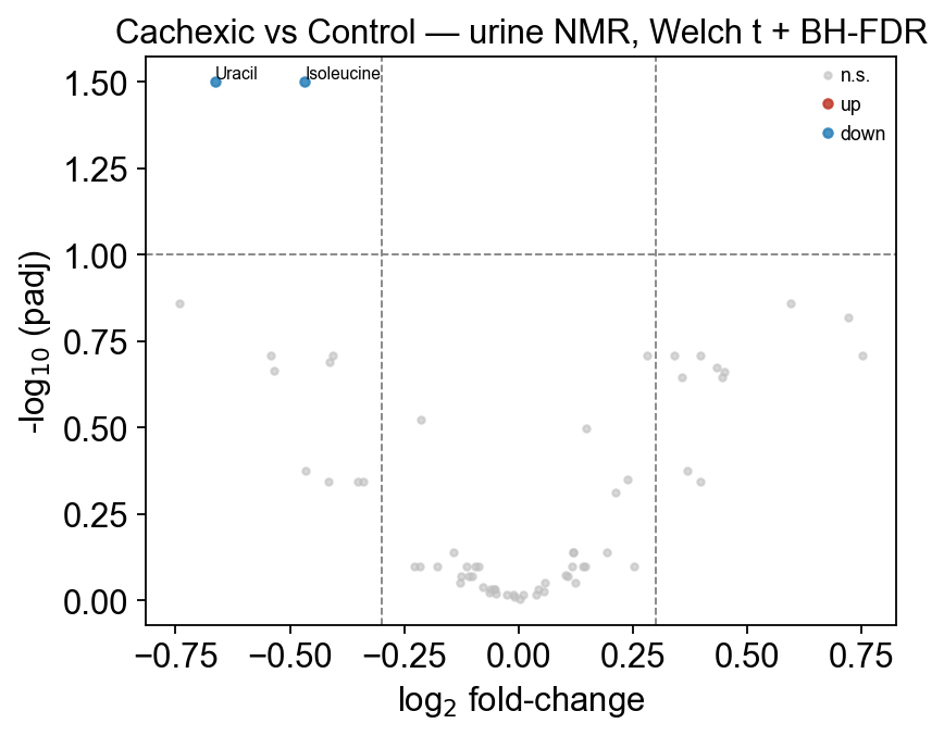
The top hits — Isoleucine, Uracil, Glucose, Acetone, Methylguanidine — are all known cachexia urinary biomarkers published in Eisner et al. 2010. The log2fc column tells you the direction: Glucose is up in cachexia (↑ in group_a), whereas Isoleucine is down (↓).

7 — Volcano plot with `ov.metabol.volcano`#

ov.metabol.volcano takes the differential DataFrame directly and produces a publication-quality -log10(padj) vs log2fc scatter with configurable thresholds and top-N labeling.

Arguments:

Argument	Meaning	Typical choice
`padj_thresh`	horizontal dashed line; hits above it are “significant”	0.05 for stringent, 0.10-0.20 for exploratory
`log2fc_thresh`	vertical dashed lines; hits must exceed this magnitude to be “biologically meaningful”	0.3-1.0 — depends on study
`label_top_n`	label the N most extreme hits	5-10 for presentations

fig, ax = ov.metabol.volcano(
    deg,
    padj_thresh=0.10,
    log2fc_thresh=0.3,
    label_top_n=8,
)
ax.set_title('Cachexic vs Control — urine NMR, Welch t + BH-FDR')
plt.tight_layout(); plt.show()

../_images/84ffe6381542af78138e76cc40494f7ba301a5fcf518507141f1306395ae0d2c.png

8 — The `pyMetabo` class — chaining it all together#

The above is the functional API — good for explicit pipelines and debugging. For end-to-end analysis omicverse also ships a class ov.metabol.pyMetabo that holds the AnnData and exposes each stage as a chainable method, keeping intermediate artifacts on the instance.

m = pyMetabo(adata)                 # .raw is frozen, .adata will evolve
 .impute(method='qrilc')            # returns self
 .normalize(method='pqn')
 .transform(method='log')           # for stats use log
 .differential(method='welch_t')    # writes .deg_table
 .transform(method='pareto',
            stash_raw=False)        # then Pareto-scale for multivariate
 .opls_da(n_ortho=1)                # writes .plsda_result

This is the same pipeline as the functional API above but with state management — useful for notebooks where you want to inspect the intermediate at every step.

m = (
    ov.metabol.pyMetabo(adata.copy())
      .normalize(method='pqn')
      .transform(method='log')
      .differential(method='welch_t', log_transformed=True)
)
# Class and functional API agree to machine precision
assert (m.deg_table['pvalue'].values == deg['pvalue'].values).all()
print('class-API and functional-API p-values match exactly ✓')
print(f'n hits at padj<0.20: {len(m.significant_metabolites(padj_thresh=0.20, log2fc_thresh=0.0))}')

class-API and functional-API p-values match exactly ✓
n hits at padj<0.20: 11

9 — What’s on the AnnData now?#

Every preprocessing step recorded itself on the AnnData so you can trace the pipeline:

print('adata.obs columns    :', list(pareto_adata.obs.columns))
print('adata.var columns    :', list(pareto_adata.var.columns))
print('adata.uns entries    :', list(pareto_adata.uns.keys()))
print('adata.uns["metabol"] :', pareto_adata.uns.get('metabol', {}))
print('adata.layers         :', list(pareto_adata.layers.keys()))

adata.obs columns    : ['group']
adata.var columns    : []
adata.uns entries    : ['metabol']
adata.uns["metabol"] : {'normalization': 'pqn', 'transform': 'pareto'}
adata.layers         : ['raw']

10 — Testing 3+ groups with `anova`#

differential covers the two-group case. When your design has three or more levels (dose-response, time series, treatment arms) use ov.metabol.anova. Three methods:

welch_anova (default) — Alexander-Govern / Welch ANOVA. Handles unequal variances; the recommended default.
anova — classic f_oneway. Fastest, assumes equal variance.
kruskal — Kruskal-Wallis. Non-parametric.

The dataset here is binary, so to demonstrate we bin Isoleucine into three dose tertiles and test the other metabolites across the tertiles. In your own work you would pass your real multi-level factor via group_col.

# Build a 3-level dose factor from Isoleucine tertiles
import pandas as pd
import numpy as np
ile = adata[:, 'Isoleucine'].X.toarray().ravel() if hasattr(adata.X, 'toarray')       else np.asarray(adata[:, 'Isoleucine'].X).ravel()
adata_mg = adata.copy()
adata_mg.obs['ile_tertile'] = pd.qcut(ile, 3, labels=['low', 'mid', 'high']).astype(str)
# Pre-process for a fair test
adata_mg = ov.metabol.impute(adata_mg, method='qrilc', seed=0)
adata_mg = ov.metabol.normalize(adata_mg, method='pqn')
adata_mg = ov.metabol.transform(adata_mg, method='log')

aov = ov.metabol.anova(adata_mg, group_col='ile_tertile',
                       method='welch_anova')
print(f'{(aov["padj"] < 0.05).sum()} features with padj<0.05 across dose tertiles')
aov.head(10)

4 features with padj<0.05 across dose tertiles

                                stat    pvalue      padj  mean_mid  mean_high  \
1,6-Anhydro-beta-D-glucose  4.257566  0.118982  0.416437  5.718287   5.894960   
1-Methylnicotinamide        0.406515  0.816068  0.886419  5.285041   5.289838   
2-Aminobutyrate             3.536946  0.170593  0.455945  3.793046   3.395891   
2-Hydroxyisobutyrate        1.655057  0.437128  0.756974  4.971272   4.883103   
2-Oxoglutarate              3.522799  0.171804  0.455945  6.106611   5.869704   
3-Aminoisobutyrate          0.564936  0.753921  0.865201  4.751072   5.086486   
3-Hydroxybutyrate           1.862893  0.393983  0.730028  3.768444   4.035600   
3-Hydroxyisovalerate        1.126824  0.569264  0.794695  3.676931   3.894236   
3-Indoxylsulfate            4.660348  0.097279  0.401639  7.357230   7.076545   
4-Hydroxyphenylacetate      2.701209  0.259084  0.562837  6.349393   6.195603   

                            mean_low  n_groups  
1,6-Anhydro-beta-D-glucose  6.398782         3  
1-Methylnicotinamide        5.445472         3  
2-Aminobutyrate             3.800911         3  
2-Hydroxyisobutyrate        5.078845         3  
2-Oxoglutarate              5.459679         3  
3-Aminoisobutyrate          4.959798         3  
3-Hydroxybutyrate           3.817724         3  
3-Hydroxyisovalerate        3.960560         3  
3-Indoxylsulfate            7.559225         3  
4-Hydroxyphenylacetate      6.524763         3  

Because we built the factor from one of the features, any metabolite correlated with Isoleucine shows up as significant — this serves as a sanity check that the ANOVA engine works. On a real dose-response study the factor would be your experimental dose column, and the same call pattern applies.

Summary#

Stage	Function	Key methodological choice
I/O	`ov.metabol.read_metaboanalyst`	standard MetaboAnalyst CSV layout
Imputation	`ov.metabol.impute`	QRILC for MNAR-heavy LC-MS, kNN for MAR
Sample normalize	`ov.metabol.normalize('pqn')`	PQN for robustness to biologically-changed features
Feature transform	`ov.metabol.transform('log')` + `.transform('pareto')`	log for stats, Pareto for multivariate
Univariate stats	`ov.metabol.differential('welch_t')`	Welch’s t default; use limma for small-n, Wilcoxon for non-normal
FDR correction	built-in BH	expect few hits at padj<0.05 on small studies
Volcano	`ov.metabol.volcano`	label top-N, dashed thresholds

Next: t_metabol_02_multivariate.ipynb — how to go from univariate volcano to PLS-DA / OPLS-DA and why the VIP score is more informative than p-value when features correlate.