Single-cell copy-number variation with inferCNV

This tutorial walks through ov.single.CNV(method='infercnv') — a wrapper around the pure-Python py-inferCNV re-implementation of the Broad Institute’s R inferCNV (Tickle et al., 2019).

inferCNV is reference-anchored: you tell it which cell-type categories to treat as diploid normals, and the resulting CN matrix is each cell’s deviation from that reference. This is more sensitive than CopyKAT when a clean normal population exists in the same dataset (e.g. immune cells in a tumour biopsy), at the cost of needing a cell-type annotation.

Why use omicverse/py-inferCNV instead of icbi-lab/infercnvpy?

infercnvpy (ICBI Lab) is a lightweight Python wrapper that re-implements R inferCNV’s Phase 1 (preprocessing) pipeline only. It explicitly omits Phases 2 and 3 — the HMM-based CNV region calling and Bayesian filtering steps that are central to R inferCNV’s scientific output. This is acknowledged by the maintainer in #1 (“HMM-based CNV caller”, open since 2021) and #121 (“stable release”, closed 2024 with “I don’t have the time to further pursue this project”). The repo has accumulated 18 open issues including long-standing gaps on gene-level CNV extraction (#50, open since 2022) and memory scaling (#180, 2026). In contrast, py-inferCNV ships Phase 2 (HMM i3/i6 state calling, tumour subclustering) and Phase 3 (BayesNet filtering, denoising) as of v0.2.0, with bit-exact R-parity validation on Phase 1 (max diff < 1e-10) and Spearman ρ = 1.0000 on Phase 2 across multiple 10x patients — see its NAMESPACE_PARITY.md for the audit table. The omicverse wrapper consumes it directly, no R needed.

Part.1 The math behind inferCNV

inferCNV’s Phase 1 pipeline:

1. Filter + normalise. Low-expression genes are dropped; counts are normalised by sequencing depth and log-transformed $\(\;\;\tilde x_{ij} = \log_2(c_{ij} + 1)\)\( where \)c_{ij}\( is the depth-normalised count of gene \)j\( in cell \)i$.

2. Reference subtraction. For each gene, the mean expression of reference cells is subtracted from every cell: $\(\;\;r_{ij} = \tilde x_{ij} - \overline{\tilde x_{j,\,\text{ref}}}.\)$

3. Pyramidal smoothing. A weighted moving average of width window_length (default 101) is applied along each chromosome to suppress per-gene noise while preserving copy-number breakpoints.

4. Centre cells. The median of each cell’s smoothed profile is subtracted so the diploid baseline sits at zero.

5. Second reference subtraction + log inversion. Repeats step 2 on the smoothed values, then maps log-ratios back through \(2^x - 1\) to yield a per-bin CN deviation.

6. Outlier pruning. Bins exceeding lfc_clip (default 3) are clipped to suppress experimental artefacts.

Reference: Patel et al., Science (2014) — original method; broadinstitute/inferCNV — R implementation.

Part.2 Load data

Maynard et al. (2020) lung adenocarcinoma, 3 000 cells. The file already carries gene-coordinate metadata in adata.var (chromosome, start, end) — inferCNV uses these to order genes along the genome.

import omicverse as ov
ov.plot_set()

🔬 Starting plot initialization...
🧬 Detecting GPU devices…
✅ NVIDIA CUDA GPUs detected: 1
    • [CUDA 0] NVIDIA H100 80GB HBM3
      Memory: 79.1 GB | Compute: 9.0

   ____            _     _    __                  
  / __ \____ ___  (_)___| |  / /__  _____________ 
 / / / / __ `__ \/ / ___/ | / / _ \/ ___/ ___/ _ \ 
/ /_/ / / / / / / / /__ | |/ /  __/ /  (__  )  __/ 
\____/_/ /_/ /_/_/\___/ |___/\___/_/  /____/\___/                                              

🔖 Version: 2.1.3rc1   📚 Tutorials: https://omicverse.readthedocs.io/
✅ plot_set complete.

import os
import scanpy as sc
import omicverse as ov

# Maynard et al. (2020) lung adenocarcinoma scRNA-seq — 3 000 cells, 55 556
# genes, gene coordinates already in adata.var. Bundled by infercnvpy.
DATA_URL = "https://github.com/icbi-lab/infercnvpy/releases/download/d0.1.0/maynard2020_3k.h5ad"
data_dir = "data/cnv"
os.makedirs(data_dir, exist_ok=True)
adata = sc.read(f"{data_dir}/maynard2020_3k.h5ad", backup_url=DATA_URL)
adata

AnnData object with n_obs × n_vars = 3000 × 55556
    obs: 'age', 'sex', 'sample', 'patient', 'cell_type'
    var: 'ensg', 'mito', 'n_cells_by_counts', 'mean_counts', 'pct_dropout_by_counts', 'total_counts', 'n_counts', 'chromosome', 'start', 'end', 'gene_id', 'gene_name'
    uns: 'cell_type_colors', 'neighbors', 'umap'
    obsm: 'X_scVI', 'X_umap'
    obsp: 'connectivities', 'distances'

Part.3 Identify reference cells

Reference cells must be biologically diploid. In a tumour biopsy the infiltrating immune cells (T cells, B cells, macrophages, monocytes, NK cells) are the canonical choice — they’re abundant, homogeneous, and near-certain to have a normal karyotype. Stromal cells (fibroblasts, endothelial) can also be used.

Here we use the four largest non-epithelial categories as references. Epithelial cells become the query (potentially aneuploid) population.

reference_cats = ['T cell CD4', 'T cell CD8', 'Macrophage', 'B cell']
print('Reference cells (diploid):',
      int(adata.obs["cell_type"].isin(reference_cats).sum()))
print('Query cells (epithelial / other):',
      int(adata.obs["cell_type"].isin(['Epithelial cell']).sum()),
      '(Epithelial cell only)')

Reference cells (diploid): 997
Query cells (epithelial / other): 522 (Epithelial cell only)

Part.4 Run inferCNV

ov.single.CNV(method='infercnv') writes the same unified schema as CopyKAT — same plot calls work unchanged.

slot	content
adata.obsm['X_cnv']	cells × ~4 k bins of log-CN
adata.uns['cnv']['chr_pos']	chromosome → starting-bin index
adata.obs['cnv_score']	per-cell mean abs(log-CN) — proxy for “tumour-ness”

inferCNV does not classify cells by default — adata.obs['cnv_prediction'] stays NaN. To threshold cnv_score into tumour/normal after the fact, see the bottom of the notebook.

cnv = ov.single.CNV(adata, method='infercnv')
cnv.run(reference_key='cell_type', reference_cat=reference_cats,
        exclude_chromosomes=('chrX', 'chrY', 'chrM'), verbose=False)

<omicverse.single._cnv.CNV at 0x7f14550906a0>

adata.obs[['cnv_score']].describe().T

	count	mean	std	min	25%	50%	75%	max
cnv_score	3000.0	0.073123	0.017058	0.028157	0.061502	0.072854	0.08243	0.233666

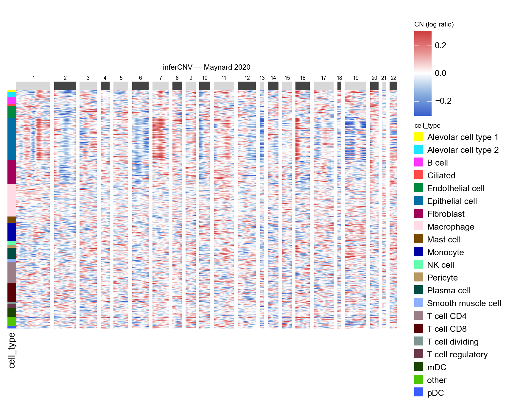
Part.5 Genome-wide heatmap

Plotting the cells grouped by their original cell_type annotation lets us see whether tumour-like CN patterns concentrate in the Epithelial-cell band. Immune and stromal cells should sit near zero (they were the reference); Epithelial cells should show recurrent gains and losses.

groupby picks a single adata.obs column for row ordering. If you want an extra colour strip on top without changing the order, pass it via annotations — see the CopyKAT tutorial for an example.

ov.pl.cnv_heatmap(adata, groupby='cell_type',
                  figsize=(8, 5), title='inferCNV — Maynard 2020')

<marsilea.heatmap.Heatmap at 0x7f14550a3e80>

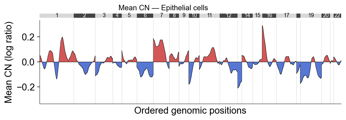
Part.6 Mean CN summary

Mean CN per bin restricted to Epithelial cells — the pseudo-bulk tumour profile.

ov.pl.cnv_summary(adata, groupby='cell_type', subset='Epithelial cell',
                  figsize=(8, 2.6), title='Mean CN — Epithelial cells')

(<Figure size 640x208 with 2 Axes>,
 {'line': <Axes: xlabel='Ordered genomic positions', ylabel='Mean CN (log ratio)'>,
  'ideogram': <Axes: >})

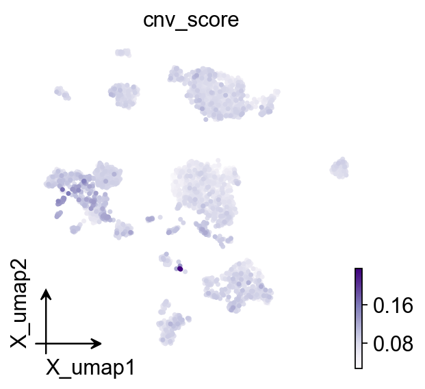
Part.7 UMAP

inferCNV doesn’t classify cells, but cnv_score (mean absolute CN deviation) is a useful continuous “tumour-ness” gradient. Overlaying it on the existing UMAP shows whether the score peaks at the Epithelial cluster.

ov.pl.cnv_umap(adata, color='cnv_score')

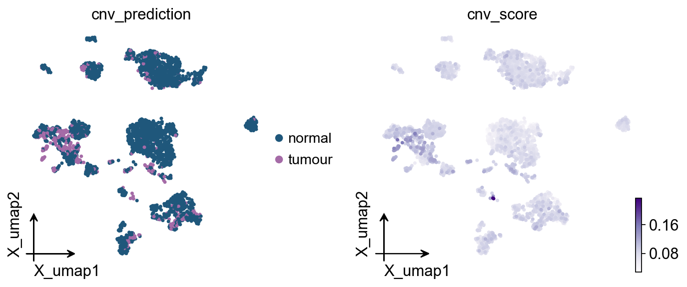
Thresholding cnv_score into a tumour / normal call

If you want a categorical call on top of inferCNV, a simple threshold on cnv_score (e.g. > 90th percentile of reference cells) works well:

import numpy as np
ref_mask = adata.obs['cell_type'].isin(reference_cats).values
ref_threshold = np.percentile(adata.obs.loc[ref_mask, 'cnv_score'], 95)
adata.obs['cnv_prediction'] = np.where(
    adata.obs['cnv_score'] > ref_threshold, 'tumour', 'normal'
)
adata.obs['cnv_prediction'] = adata.obs['cnv_prediction'].astype('category')
adata.obs['cnv_prediction'].value_counts()

cnv_prediction
normal    2544
tumour     456
Name: count, dtype: int64

ov.pl.cnv_umap(adata, color=['cnv_prediction', 'cnv_score'])

---

Next steps: for unsupervised CN inference (no reference annotation needed), see the CopyKAT tutorial. The two methods can disagree at the margins — running both on the same dataset and comparing their cnv_score columns side-by-side (ov.pl.embedding(adata, color=['cnv_score_copykat', 'cnv_score_infercnv'])) is a useful sanity check.