Batch effect and drift correction for LC-MS#
LC-MS untargeted runs suffer from two kinds of unwanted variation that ComBat alone cannot handle:
Signal drift within a batch — the injection-time-dependent decay of signal due to source fouling, column aging, etc. Drift is continuous in injection order, not categorical.
Batch shifts between batches — quantified by ComBat when the batch variable is known.
This tutorial shows the recommended combo on a synthetic LC-MS run with planted drift + QC pool samples. Synthetic data lets us verify that correction works before you apply it to your own study.
Pipeline:
ov.metabol.drift_correct— per-feature LOESS fit on QC injection orderov.metabol.serrf— QC-based Random Forest (Fan 2019) that borrows strength from correlated co-featuresov.bulk.batch_correction— ComBat for residual between-batch shifts
0 — Setup and simulated LC-MS run#
Simulate 60 samples over 2 batches with 10 QC samples per batch, 40 features. First 15 features have a time-dependent exponential drift; real samples have a small case/ctrl effect on features 20–24.
import numpy as np
import pandas as pd
import matplotlib.pyplot as plt
from anndata import AnnData
import omicverse as ov

rng = np.random.default_rng(0)

n_real_per_batch = 20
n_qc_per_batch = 10
n_batches = 2
n_features = 40
drift_features = 15
drift_strength = 1.5

rows, idx = [], []
order = 0
for b in range(n_batches):
    plan = ['QC']*n_qc_per_batch + ['real']*n_real_per_batch
    rng.shuffle(plan)
    for k, kind in enumerate(plan):
        rows.append({
            'sample_type': kind,
            'group': 'QC' if kind == 'QC' else ('case' if rng.random() > 0.5 else 'ctrl'),
            'batch': f'b{b}',
            'order': order,
        })
        idx.append(f'b{b}_s{k}')
        order += 1

obs = pd.DataFrame(rows, index=idx)
n = len(obs)

# Baseline signal + drift
X = rng.lognormal(mean=4.0, sigma=0.3, size=(n, n_features))
max_order = float(obs['order'].max())
t = obs['order'].to_numpy() / max_order
X[:, :drift_features] *= np.exp(drift_strength * t)[:, None]

# Inject a between-batch additive shift on features 30-39 (ComBat target)
b_mask = (obs['batch'] == 'b1').to_numpy()
X[b_mask, 30:] *= 1.4

# Tiny biology effect on features 20-24
case = (obs['group'] == 'case').to_numpy()
X[case, 20:25] *= 1.8

var = pd.DataFrame(index=[f'feat{i}' for i in range(n_features)])
adata = AnnData(X=X, obs=obs, var=var)
adata.shape
(60, 40)
1 — Baseline: QC CV% before any correction#
Features with drift should have inflated CV% on the pool of QC samples — that is the diagnostic we use to evaluate every correction step.
def qc_cv_pct(adata, qc_col='sample_type', qc_label='QC', layer=None):
    mask = (adata.obs[qc_col] == qc_label).to_numpy()
    X = adata.X if layer is None else adata.layers[layer]
    X = np.asarray(X)[mask]
    mu = X.mean(axis=0)
    sd = X.std(axis=0, ddof=1)
    return np.where(mu > 0, 100 * sd / mu, np.nan)

cv_raw = qc_cv_pct(adata)
print(f'Before correction — drift features mean CV: {cv_raw[:drift_features].mean():.1f}%')
print(f'                  stable features mean CV: {cv_raw[drift_features:30].mean():.1f}%')
Before correction — drift features mean CV: 52.7%
                  stable features mean CV: 27.0%
2 — Step 1: per-feature LOESS drift correction#
drift_correct fits a LOESS curve through the QC samples on each
feature (independently) and divides every sample’s value by that
fitted curve. This is the classic first-pass correction.
adata_drift = ov.metabol.drift_correct(
    adata,
    injection_order='order',
    qc_mask=(adata.obs['sample_type'] == 'QC').to_numpy(),
)
cv_drift = qc_cv_pct(adata_drift)
print(f'After drift_correct — drift features CV: {cv_drift[:drift_features].mean():.1f}%')
After drift_correct — drift features CV: 27.9%
3 — Step 2: SERRF#
serrf borrows strength from correlated co-features to model each
feature’s expected QC baseline. For drifts that are not monotonic
(e.g. dips + recoveries) SERRF catches what LOESS cannot.
SERRF stores the original matrix in .layers['raw'] and per-feature
CV% before/after in .var:
adata_serrf = ov.metabol.serrf(
    adata,
    qc_col='sample_type', qc_label='QC',
    batch_col='batch',
    top_k=8, n_estimators=100, seed=0,
)

summary = pd.DataFrame({
    'CV_raw': adata_serrf.var['cv_qc_raw'],
    'CV_serrf': adata_serrf.var['cv_qc_serrf'],
})
summary['improvement_%'] = (summary['CV_raw'] - summary['CV_serrf']) / summary['CV_raw'] * 100
summary.head(15)
           CV_raw   CV_serrf  improvement_%
feat0   56.712720  41.317210      27.146485
feat1   50.464151  41.509849      17.743888
feat2   51.106795  28.093674      45.029473
feat3   57.893748  41.949325      27.540836
feat4   54.810053  42.488580      22.480315
feat5   66.226161  43.664605      34.067438
feat6   49.466170  30.746594      37.843189
feat7   46.728802  36.454210      21.987707
feat8   63.352723  32.301074      49.013913
feat9   58.121089  39.154273      32.633276
feat10  53.929962  36.316246      32.660353
feat11  39.701253  30.850989      22.292154
feat12  41.694817  32.690616      21.595491
feat13  50.296132  37.530333      25.381274
feat14  49.698648  29.473423      40.695725
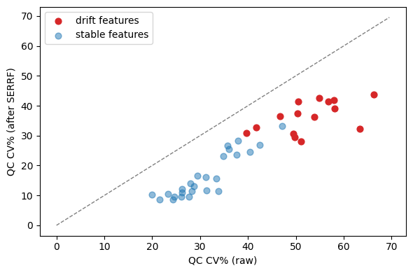
Plot CV% before vs after SERRF on drift features:
fig, ax = plt.subplots(figsize=(6, 4))
is_drift = np.arange(n_features) < drift_features
ax.scatter(summary['CV_raw'][is_drift], summary['CV_serrf'][is_drift],
           color='C3', label='drift features', s=40)
ax.scatter(summary['CV_raw'][~is_drift], summary['CV_serrf'][~is_drift],
           color='C0', label='stable features', s=40, alpha=0.5)
lim = max(summary['CV_raw'].max(), summary['CV_serrf'].max()) * 1.05
ax.plot([0, lim], [0, lim], '--', color='gray', lw=1)
ax.set_xlabel('QC CV% (raw)')
ax.set_ylabel('QC CV% (after SERRF)')
ax.legend()
fig.tight_layout()
plt.show()
4 — Step 3: ComBat for between-batch shifts#
SERRF corrects within-batch drift but assumes you already dealt with
discrete batch shifts. We use ov.bulk.batch_correction (which wraps
combat.pycombat) for that. It works on any AnnData with a batch
column.
ov.bulk.batch_correction(adata_serrf, batch_key='batch',
                           key_added='batch_correction')
print('ComBat output in adata_serrf.layers["batch_correction"]')
print('shape:', adata_serrf.layers['batch_correction'].shape)
Found 2 batches.
Adjusting for 0 covariate(s) or covariate level(s).
Standardizing Data across genes.
Fitting L/S model and finding priors.
Finding parametric adjustments.
Adjusting the Data
Storing batch correction result in adata.layers['batch_correction']
ComBat output in adata_serrf.layers["batch_correction"]
shape: (60, 40)
5 — Sample-level outlier detection (sample_qc)#
QC / batch correction assumes your samples are themselves usable. A
single mis-injected or contaminated sample can dominate a PLS-DA
component and hide real biology. ov.metabol.sample_qc fits PCA on
adata.X and returns two SIMCA-style diagnostics:
Hotelling T² — distance inside the PCA model. Flags unusual but within-model profiles.
DModX — distance to the residual plane. Flags novel profiles that don’t fit the PCA subspace at all.
A sample flagged by either metric deserves a look before downstream stats. Run on the SERRF-corrected real samples (QC pools excluded):
real_mask = (adata_serrf.obs['sample_type'] == 'real').to_numpy()
adata_real = adata_serrf[real_mask].copy()

qc_diag = ov.metabol.sample_qc(adata_real, n_components=3, alpha=0.95)
print(f'{qc_diag["is_outlier"].sum()} outlier sample(s) out of {len(qc_diag)}')
qc_diag.sort_values('T2', ascending=False).head(10)
8 outlier sample(s) out of 40
              T2     DModX   T2_crit  DModX_crit  T2_flag  DModX_flag  \
b1_s6   9.214746  0.615842  9.039977    0.889306     True       False
b1_s2   7.518378  0.670938  9.039977    0.889306    False       False
b1_s15  6.808285  0.676331  9.039977    0.889306    False       False
b1_s24  5.191500  0.986138  9.039977    0.889306    False        True
b1_s8   4.994036  0.926844  9.039977    0.889306    False        True
b1_s26  4.939299  0.788794  9.039977    0.889306    False       False
b0_s1   4.724327  0.799997  9.039977    0.889306    False       False
b0_s3   4.563427  0.737520  9.039977    0.889306    False       False
b1_s0   3.888096  0.869859  9.039977    0.889306    False       False
b0_s13  3.760173  0.625570  9.039977    0.889306    False       False

        is_outlier
b1_s6         True
b1_s2        False
b1_s15       False
b1_s24        True
b1_s8         True
b1_s26       False
b0_s1        False
b0_s3        False
b1_s0        False
b0_s13       False
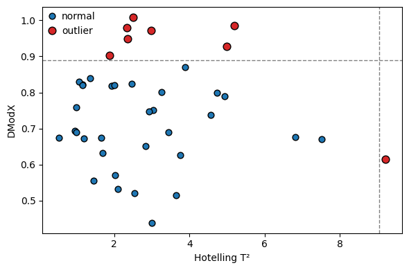
T² vs DModX scatter#
Quadrants of this plot tell you why a sample is outlying:
Top-right (high T², high DModX) — the strongest outlier kind.
Top-left — fits the model but at its edge.
Bottom-right — doesn’t fit the model; novel pattern.
fig, ax = plt.subplots(figsize=(6, 4))
flag = qc_diag['is_outlier'].to_numpy()
ax.scatter(qc_diag['T2'][~flag], qc_diag['DModX'][~flag],
           color='C0', edgecolor='k', s=40, label='normal')
ax.scatter(qc_diag['T2'][flag], qc_diag['DModX'][flag],
           color='C3', edgecolor='k', s=60, label='outlier')
ax.axvline(qc_diag['T2_crit'].iloc[0], color='gray', ls='--', lw=1)
ax.axhline(qc_diag['DModX_crit'].iloc[0], color='gray', ls='--', lw=1)
ax.set_xlabel('Hotelling T²')
ax.set_ylabel('DModX')
ax.legend()
fig.tight_layout()
plt.show()
Summary#
For a typical LC-MS study the recommended order is:
adata = ov.metabol.drift_correct(adata, injection_order=..., qc_mask=...)
adata = ov.metabol.serrf(adata, qc_col=..., batch_col=...)
ov.bulk.batch_correction(adata, batch_key=...)    # if needed
After this, standard downstream steps (impute, normalize,
transform, differential, plsda/opls_da, MSEA) apply without
modification.