Spatial deconvolution with reference scRNA-seq#
This notebook presents a fully reproducible workflow for spot-based spatial deconvolution using the unified API omicverse.space.Deconvolution, integrating Tangram and cell2location. It follows a Nature Protocol–style structure with clear purpose, inputs/outputs, parameters, timing, saving, and troubleshooting.
Audience: Bioinformatics practitioners with basic Python/Scanpy familiarity.
Data types: 10x Visium or similar spot-based spatial transcriptomics; a matched scRNA-seq reference from the same tissue/region.
Outcomes: Spot-level cell-type composition/intensity maps, trained models for reuse, and publication-ready figures.
Reproducible Environment (recommended)#
Python: ≥ 3.9 (3.10/3.11 recommended)
omicverse: pinned to the version used in this notebook
Key dependencies: scanpy, anndata, numpy, pandas, torch (GPU recommended for cell2location)
Hardware: ≥ 16 GB RAM; a CUDA-capable GPU significantly speeds cell2location
Reproducibility: set global random seeds (numpy/torch) and pin package versions.
Inputs and Outputs#
Inputs:
scRNA-seq reference with clear cell-type annotations (gene IDs harmonized, preferably ENSEMBL)
Spatial transcriptomics counts (e.g., 10x Space Ranger outputs) from matched tissue/region
Outputs:
Deconvolution matrices and cell-type spatial intensity/probability maps
Saved models/parameters for quick reload and reuse
Key figures: spatial heatmaps, multi-target overlays, local pie charts
Workflow Overview with Estimated Timing#
Prepare scRNA-seq reference (10–20 min)
Prepare spatial transcriptomics (10–20 min)
Tangram deconvolution: preprocess → fit → save/reuse (15–30 min)
cell2location: reference learning → spatial mapping → save/reuse (30–120 min; GPU faster)
Visualization and export (5–15 min)
Tip: Each step below documents purpose, inputs/outputs, and critical parameters to support reproducibility and adaptation to your data.
import squidpy as sq

import omicverse as ov
#print(f"omicverse version: {ov.__version__}")
import scanpy as sc
#print(f"scanpy version: {sc.__version__}")
ov.plot_set(font_path='Arial')

# Enable auto-reload for development
%load_ext autoreload
%autoreload 2
🔬 Starting plot initialization...
Using already downloaded Arial font from: /tmp/omicverse_arial.ttf
Registered as: Arial
🧬 Detecting GPU devices…
✅ NVIDIA CUDA GPUs detected: 1
    • [CUDA 0] NVIDIA H100 80GB HBM3
      Memory: 79.1 GB | Compute: 9.0

   ____            _     _    __
  / __ \____ ___  (_)___| |  / /__  _____________
 / / / / __ `__ \/ / ___/ | / / _ \/ ___/ ___/ _ \
/ /_/ / / / / / / / /__ | |/ /  __/ /  (__  )  __/
\____/_/ /_/ /_/_/\___/ |___/\___/_/  /____/\___/

🔖 Version: 1.7.8rc1   📚 Tutorials: https://omicverse.readthedocs.io/
✅ plot_set complete.
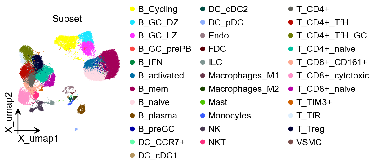
Step 1: Prepare the scRNA-seq reference (1 min)#
Purpose: load and standardize the single-cell reference ensuring consistent cell-type annotations and harmonized gene IDs (prefer ENSEMBL).
Inputs: public lymph node/spleen/tonsil scRNA-seq or your own dataset
Outputs:
AnnDataobject (adata_ref) with normalized variable names and cell-type annotationsKey points:
The reference should cover major cell types/states expected in the spatial sample.
Harmonize gene IDs with the spatial data (ENSEMBL or symbols) to avoid failed mappings.
adata_sc = ov.datasets.sc_ref_Lymph_Node()
import matplotlib.pyplot as plt
fig, ax = plt.subplots(figsize=(3,3))
ov.utils.embedding(
    adata_sc,
    basis="X_umap",
    color=['Subset'],
    title='Subset',
    frameon='small',
    #ncols=1,
    wspace=0.65,
    #palette=ov.utils.pyomic_palette()[11:],
    show=False,
    ax=ax
)
<Axes: title={'center': 'Subset'}, xlabel='X_umap1', ylabel='X_umap2'>
Step 2: Prepare spatial transcriptomics (1 min)#
Purpose: load 10x Visium (Space Ranger outputs) or similar to obtain a coordinate-aware spatial AnnData (adata_sp).
Inputs: Visium count matrix and spatial coordinates (from the
spatialfolder)Outputs:
AnnDataobject (adata_sp) with spot coordinates and countsKey points:
Ensure maximal gene overlap with the scRNA-seq reference; map gene IDs if necessary.
For multiple samples, keep batch labels explicit to support merging and visualization.
adata_sp = sc.datasets.visium_sge(sample_id="V1_Human_Lymph_Node")
adata_sp.obs['sample'] = list(adata_sp.uns['spatial'].keys())[0]
adata_sp.var_names_make_unique()
reading /scratch/users/steorra/analysis/omic_test/data/V1_Human_Lymph_Node/filtered_feature_bc_matrix.h5
 (0:00:00)
Step 3: Tangram deconvolution (15–30 min)#
Tangram maps scRNA-seq expression into spatial coordinates to infer cell-type distribution and proportions. We use omicverse.space.Deconvolution for a consistent interface.
decov_obj=ov.space.Deconvolution(
    adata_sc=adata_sc,
    adata_sp=adata_sp
)
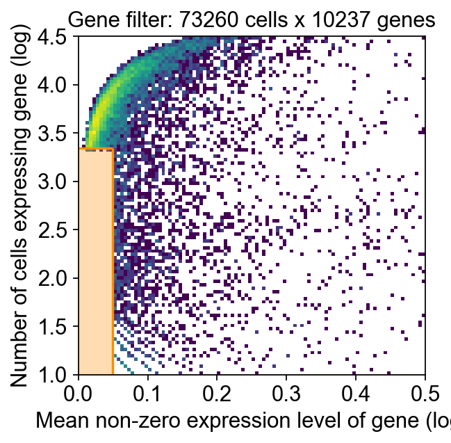
Step 3.1 Tangram preprocessing#
Purpose: prepare scRNA-seq and spatial data with necessary filtering/transformations to enable robust fitting (prefer raw counts).
decov_obj.preprocess_sc(
    mode='shiftlog|pearson',n_HVGs=3000,target_sum=1e4,
)
decov_obj.preprocess_sp(
    mode='pearsonr',n_svgs=3000,target_sum=1e4,
)
🔍 [2025-09-20 03:25:56] Running preprocessing in 'cpu' mode...
Begin robust gene identification
    After filtration, 10237/10237 genes are kept.
    Among 10237 genes, 9838 genes are robust.
✅ Robust gene identification completed successfully.
Begin size normalization: shiftlog and HVGs selection pearson

🔍 Count Normalization:
   Target sum: 10000.0
   Exclude highly expressed: True
   Max fraction threshold: 0.2
   ⚠️ Excluding 17 highly-expressed genes from normalization computation

✅ Count Normalization Completed Successfully!
   ✓ Processed: 73,260 cells × 9,838 genes
   ✓ Runtime: 2.70s

🔍 Highly Variable Genes Selection (Experimental):
   Method: pearson_residuals
   Target genes: 3,000
   Theta (overdispersion): 100

✅ Experimental HVG Selection Completed Successfully!
   ✓ Selected: 3,000 highly variable genes out of 9,838 total (30.5%)
   ✓ Results added to AnnData object:
     • 'highly_variable': Boolean vector (adata.var)
     • 'highly_variable_rank': Float vector (adata.var)
     • 'highly_variable_nbatches': Int vector (adata.var)
     • 'highly_variable_intersection': Boolean vector (adata.var)
     • 'means': Float vector (adata.var)
     • 'variances': Float vector (adata.var)
     • 'residual_variances': Float vector (adata.var)
    Time to analyze data in cpu: 10.15 seconds.
✅ Preprocessing completed successfully.
    Added:
        'highly_variable_features', boolean vector (adata.var)
        'means', float vector (adata.var)
        'variances', float vector (adata.var)
        'residual_variances', float vector (adata.var)
        'counts', raw counts layer (adata.layers)
    End of size normalization: shiftlog and HVGs selection pearson
✓ scRNA-seq data is preprocessed
🔍 [2025-09-20 03:26:10] Running preprocessing in 'cpu' mode...
Begin robust gene identification
    After filtration, 25187/36601 genes are kept.
    Among 25187 genes, 22411 genes are robust.
✅ Robust gene identification completed successfully.
Begin size normalization: shiftlog and HVGs selection pearson

🔍 Count Normalization:
   Target sum: 10000.0
   Exclude highly expressed: True
   Max fraction threshold: 0.2
   ⚠️ Excluding 1 highly-expressed genes from normalization computation
   Excluded genes: ['IGKC']

✅ Count Normalization Completed Successfully!
   ✓ Processed: 4,035 cells × 22,411 genes
   ✓ Runtime: 0.44s

🔍 Highly Variable Genes Selection (Experimental):
   Method: pearson_residuals
   Target genes: 3,000
   Theta (overdispersion): 100

✅ Experimental HVG Selection Completed Successfully!
   ✓ Selected: 3,000 highly variable genes out of 22,411 total (13.4%)
   ✓ Results added to AnnData object:
     • 'highly_variable': Boolean vector (adata.var)
     • 'highly_variable_rank': Float vector (adata.var)
     • 'highly_variable_nbatches': Int vector (adata.var)
     • 'highly_variable_intersection': Boolean vector (adata.var)
     • 'means': Float vector (adata.var)
     • 'variances': Float vector (adata.var)
     • 'residual_variances': Float vector (adata.var)
    Time to analyze data in cpu: 2.04 seconds.
✅ Preprocessing completed successfully.
    Added:
        'highly_variable_features', boolean vector (adata.var)
        'means', float vector (adata.var)
        'variances', float vector (adata.var)
        'residual_variances', float vector (adata.var)
        'counts', raw counts layer (adata.layers)
    End of size normalization: shiftlog and HVGs selection pearson
✓ spatial transcriptomics data is preprocessed
Step 3.2 Run Tangram deconvolution (see above for I/O and parameters)#
decov_obj.deconvolution(
    method='Tangram',celltype_key_sc='Subset',
    tangram_kwargs={'mode':'cells','num_epochs':500,'device':'cuda:0'}
)
tangram have been install version: 1.0.4
ranking genes
    finished: added to `.uns['Subset_rank_genes_groups']`
    'names', sorted np.recarray to be indexed by group ids
    'scores', sorted np.recarray to be indexed by group ids
    'logfoldchanges', sorted np.recarray to be indexed by group ids
    'pvals', sorted np.recarray to be indexed by group ids
    'pvals_adj', sorted np.recarray to be indexed by group ids (0:00:04)
...Calculate The Number of Markers: 1290
INFO:root:832 training genes are saved in `uns``training_genes` of both single cell and spatial Anndatas.
INFO:root:1291 overlapped genes are saved in `uns``overlap_genes` of both single cell and spatial Anndatas.
INFO:root:uniform based density prior is calculated and saved in `obs``uniform_density` of the spatial Anndata.
INFO:root:rna count based density prior is calculated and saved in `obs``rna_count_based_density` of the spatial Anndata.
...Model prepared successfully
INFO:root:Allocate tensors for mapping.
INFO:root:Begin training with 832 genes and rna_count_based density_prior in cells mode...
INFO:root:Printing scores every 100 epochs.
Score: 0.814, KL reg: 0.002
Score: 0.911, KL reg: 0.000
Score: 0.929, KL reg: 0.000
Score: 0.934, KL reg: 0.000
Score: 0.935, KL reg: 0.000
INFO:root:Saving results..
AnnData object with n_obs × n_vars = 73260 × 4035
    obs: 'Age', 'BCELL_CLONE', 'BCELL_CLONE_SIZE', 'Donor', 'ID', 'IGH_MU_FREQ', 'ISOTYPE', 'LibraryID', 'Method', 'Population', 'PrelimCellType', 'Sample', 'Sex', 'Study', 'Tissue', 'barcode', 'batch', 'doublet_score', 'index', 'predicted_doublet', 'percent_mito', 'n_counts', 'n_genes', 'S_score', 'G2M_score', 'phase', 'VDJsum', 'cell_cycle_diff', 'PrelimCellType_new', 'leiden', 'leiden_1', 'leiden_2', 'leiden_3', 'leiden_4', 'CellType', 'CellType2', 'Subset', 'Subset_Broad', 'Subset_all', 'new_celltype', 'Subset_int', 'Subset_print'
    var: 'in_tissue', 'array_row', 'array_col', 'sample', 'uniform_density', 'rna_count_based_density'
    uns: 'train_genes_df', 'training_history'
INFO:root:spatial prediction dataframe is saved in `obsm` `tangram_ct_pred` of the spatial AnnData.
...Model train successfully
✓ Tangram cell2location is done
The cell2location result is saved in self.adata_cell2location
<omicverse.space._tangram.Tangram at 0x7f8bad6cbca0>
Step 3.3 Save Tangram model and results (<1 min)#
Recommended artifacts to save:
Fitted mapping/probability matrices
Core hyperparameters and software versions (for reproducibility)
Result
AnnData/DataFramefor downstream plotting
ov.utils.save(
    decov_obj.tangram_model,
    'result/model/tangram_model.pkl'
)
💾 Save Operation:
   Target path: result/model/tangram_model.pkl
   Object type: Tangram
   Using: pickle
   Pickle failed, switching to: cloudpickle
   ✅ Successfully saved using cloudpickle!
────────────────────────────────────────────────────────────
decov_obj.adata_sc.write(f"result/model/tangram_adata_sc.h5ad")
decov_obj.adata_sp.write(f"result/model/tangram_adata_sp.h5ad")
Step 3.4 Result object: cell locations#
In omicverse, cell location/intensity outputs are accessible via the decov_obj container (e.g., decov_obj.adata_cell2location or related fields). Check the actual attributes in your session for where Tangram exports are stored.
decov_obj.adata_cell2location
AnnData object with n_obs × n_vars = 4035 × 3000
    obs: 'in_tissue', 'array_row', 'array_col', 'sample', 'uniform_density', 'rna_count_based_density', 'T_CD4+_naive', 'DC_cDC1', 'T_TIM3+', 'Macrophages_M2', 'T_TfR', 'T_CD8+_naive', 'Endo', 'B_activated', 'T_CD8+_CD161+', 'T_CD4+_TfH', 'FDC', 'T_Treg', 'B_plasma', 'T_CD4+', 'B_GC_LZ', 'T_CD8+_cytotoxic', 'B_GC_DZ', 'VSMC', 'B_IFN', 'B_preGC', 'B_naive', 'Macrophages_M1', 'DC_CCR7+', 'B_mem', 'ILC', 'DC_cDC2', 'B_GC_prePB', 'Mast', 'DC_pDC', 'NKT', 'Monocytes', 'B_Cycling', 'T_CD4+_TfH_GC', 'NK'
    var: 'gene_ids', 'feature_types', 'genome', 'n_cells', 'percent_cells', 'robust', 'means', 'variances', 'residual_variances', 'highly_variable_rank', 'highly_variable_features', 'space_variable_features', 'highly_variable', 'sparsity'
    uns: 'spatial', 'log1p', 'hvg', 'status', 'status_args', 'REFERENCE_MANU', 'training_genes', 'overlap_genes'
    obsm: 'spatial', 'tangram_ct_pred'
    layers: 'counts'
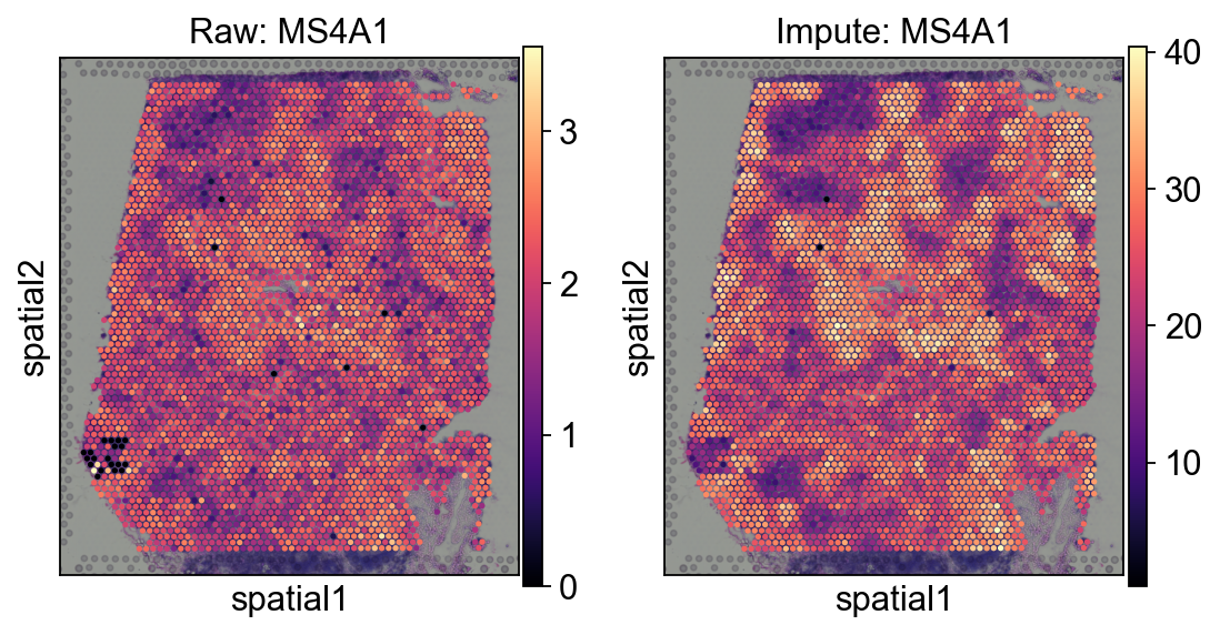
Step 3.5 Reuse: reload a saved Tangram model and impute#
Purpose: skip retraining by loading a previously saved model/matrix and performing inference on the same or similar data.
decov_obj=ov.space.Deconvolution(
    adata_sc=ov.read(f"result/model/tangram_adata_sc.h5ad"),
    adata_sp=ov.read(f"result/model/tangram_adata_sp.h5ad")
)
decov_obj.load_tangram_model(
    'result/model/tangram_model.pkl'
)
decov_obj.tangram_inference()
decov_obj.impute(method='Tangram')
decov_obj.adata_impute
✓ Existing 'counts' layer in scRNA-seq data
✓ Existing 'counts' layer in spatial transcriptomics data
✓ spatial transcriptomics data is log-normalized by 1e4
⚠️ 1e4 is the standardized target sum for `scanpy`
✓ scRNA-seq data is log-normalized by 50*1e4
✓ spatial transcriptomics data is log-normalized by 50*1e4
⚠️ 50*1e4 is the standardized target sum for `omicverse`
📂 Load Operation:
   Source path: result/model/tangram_model.pkl
   Using: pickle
   ✅ Successfully loaded!
   Loaded object type: Tangram
────────────────────────────────────────────────────────────
✓ Tangram model is loaded
The Tangram model is saved in self.tangram
✓ Tangram is done
The Tangram result is saved in self.adata_cell2location
✓ Tangram impute is done
The impute result is saved in self.adata_impute
AnnData object with n_obs × n_vars = 4035 × 3000
    obs: 'in_tissue', 'array_row', 'array_col', 'sample', 'uniform_density', 'rna_count_based_density'
    var: 'GeneID-2', 'GeneName-2', 'feature_types', 'feature_types-0', 'feature_types-1', 'gene_ids-1', 'gene_ids-4861STDY7135913-0', 'gene_ids-4861STDY7135914-0', 'gene_ids-4861STDY7208412-0', 'gene_ids-4861STDY7208413-0', 'gene_ids-Human_colon_16S7255677-0', 'gene_ids-Human_colon_16S7255678-0', 'gene_ids-Human_colon_16S8000484-0', 'gene_ids-Pan_T7935494-0', 'genome-1', 'n_cells', 'nonz_mean', 'mean_cov_effect_Subset_B_Cycling', 'mean_cov_effect_Subset_B_GC_DZ', 'mean_cov_effect_Subset_B_GC_LZ', 'mean_cov_effect_Subset_B_GC_prePB', 'mean_cov_effect_Subset_B_IFN', 'mean_cov_effect_Subset_B_activated', 'mean_cov_effect_Subset_B_mem', 'mean_cov_effect_Subset_B_naive', 'mean_cov_effect_Subset_B_plasma', 'mean_cov_effect_Subset_B_preGC', 'mean_cov_effect_Subset_DC_CCR7+', 'mean_cov_effect_Subset_DC_cDC1', 'mean_cov_effect_Subset_DC_cDC2', 'mean_cov_effect_Subset_DC_pDC', 'mean_cov_effect_Subset_Endo', 'mean_cov_effect_Subset_FDC', 'mean_cov_effect_Subset_ILC', 'mean_cov_effect_Subset_Macrophages_M1', 'mean_cov_effect_Subset_Macrophages_M2', 'mean_cov_effect_Subset_Mast', 'mean_cov_effect_Subset_Monocytes', 'mean_cov_effect_Subset_NK', 'mean_cov_effect_Subset_NKT', 'mean_cov_effect_Subset_T_CD4+', 'mean_cov_effect_Subset_T_CD4+_TfH', 'mean_cov_effect_Subset_T_CD4+_TfH_GC', 'mean_cov_effect_Subset_T_CD4+_naive', 'mean_cov_effect_Subset_T_CD8+_CD161+', 'mean_cov_effect_Subset_T_CD8+_cytotoxic', 'mean_cov_effect_Subset_T_CD8+_naive', 'mean_cov_effect_Subset_T_TIM3+', 'mean_cov_effect_Subset_T_TfR', 'mean_cov_effect_Subset_T_Treg', 'mean_cov_effect_Subset_VSMC', 'mean_sample_effectSample_4861STDY7135913', 'mean_sample_effectSample_4861STDY7135914', 'mean_sample_effectSample_4861STDY7208412', 'mean_sample_effectSample_4861STDY7208413', 'mean_sample_effectSample_4861STDY7462253', 'mean_sample_effectSample_4861STDY7462254', 'mean_sample_effectSample_4861STDY7462255', 'mean_sample_effectSample_4861STDY7462256', 'mean_sample_effectSample_4861STDY7528597', 'mean_sample_effectSample_4861STDY7528598', 'mean_sample_effectSample_4861STDY7528599', 'mean_sample_effectSample_4861STDY7528600', 'mean_sample_effectSample_BCP002_Total', 'mean_sample_effectSample_BCP003_Total', 'mean_sample_effectSample_BCP004_Total', 'mean_sample_effectSample_BCP005_Total', 'mean_sample_effectSample_BCP006_Total', 'mean_sample_effectSample_BCP008_Total', 'mean_sample_effectSample_BCP009_Total', 'mean_sample_effectSample_Human_colon_16S7255677', 'mean_sample_effectSample_Human_colon_16S7255678', 'mean_sample_effectSample_Human_colon_16S8000484', 'mean_sample_effectSample_Pan_T7935494', 'percent_cells', 'robust', 'means', 'variances', 'residual_variances', 'highly_variable_rank', 'highly_variable_features', 'sparsity', 'is_training'
    uns: 'Age_colors', 'Donor_colors', 'LibraryID_colors', 'Method_colors', 'Study_colors', 'Subset_Broad_colors', 'Subset_colors', 'Tissue_colors', 'leiden', 'neighbors', 'pca', 'phase_colors', 'regression_mod', 'umap', 'log1p', 'hvg', 'status', 'status_args', 'REFERENCE_MANU', 'Subset_rank_genes_groups', 'training_genes', 'overlap_genes'
decov_obj.adata_impute.uns=decov_obj.adata_sp.uns.copy()
decov_obj.adata_impute.obsm=decov_obj.adata_sp.obsm.copy()
#fig = ov.plt.figure(figsize=(4, 4))
fig, axes = ov.plt.subplots(1,2,figsize=(8, 4))
sc.pl.spatial(
    decov_obj.adata_sp,
    cmap='magma',
    color='MS4A1',
    ncols=4, size=1.3,ax=axes[0],
    img_key='hires',show=False,
)
axes[0].set_title('Raw: MS4A1')

sc.pl.spatial(
    decov_obj.adata_impute,
    cmap='magma',
    color='ms4a1',
    ncols=4, size=1.3,ax=axes[1],
    img_key='hires',show=False,
)
axes[1].set_title('Impute: MS4A1')
Text(0.5, 1.0, 'Impute: MS4A1')
Step 4: cell2location deconvolution (30–120 min, GPU recommended)#
cell2location is a Bayesian model that resolves fine-grained cell types in space. It typically proceeds in two stages:
learn reference signatures from scRNA-seq; 2) map those signatures to the spatial sample to estimate cell-type abundances.
adata_sc = ov.datasets.sc_ref_Lymph_Node()
adata_sp = sc.datasets.visium_sge(sample_id="V1_Human_Lymph_Node")
adata_sp.obs['sample'] = list(adata_sp.uns['spatial'].keys())[0]
adata_sp.var_names_make_unique()
reading /scratch/users/steorra/analysis/omic_test/data/V1_Human_Lymph_Node/filtered_feature_bc_matrix.h5
 (0:00:00)
decov_obj=ov.space.Deconvolution(
    adata_sc=adata_sc,
    adata_sp=adata_sp
)
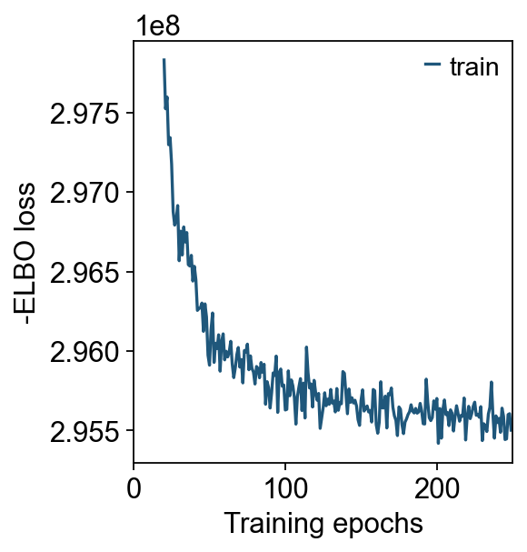
Step 4.1 Run Cell2location#
decov_obj.deconvolution(
    method='cell2location',celltype_key_sc='Subset',
    batch_key_sc=None,batch_key_sp='sample',
    cell2location_scrna_kwargs={'max_epochs':200,'batch_size':2500,'train_size':1,'lr':0.002},
    cell2location_spatial_kwargs={'max_epochs':20000,'batch_size':None,'train_size':1},
    sample_kwargs={"num_samples": 1000, "batch_size": 2500}
)
INFO:lightning.pytorch.utilities.rank_zero:GPU available: True (cuda), used: True
INFO:lightning.pytorch.utilities.rank_zero:TPU available: False, using: 0 TPU cores
INFO:lightning.pytorch.utilities.rank_zero:HPU available: False, using: 0 HPUs
INFO:lightning.pytorch.utilities.rank_zero:You are using a CUDA device ('NVIDIA H100 80GB HBM3') that has Tensor Cores. To properly utilize them, you should set `torch.set_float32_matmul_precision('medium' | 'high')` which will trade-off precision for performance. For more details, read https://pytorch.org/docs/stable/generated/torch.set_float32_matmul_precision.html#torch.set_float32_matmul_precision
INFO:lightning.pytorch.accelerators.cuda:LOCAL_RANK: 0 - CUDA_VISIBLE_DEVICES: [0]
INFO:lightning.pytorch.utilities.rank_zero:`Trainer.fit` stopped: `max_epochs=200` reached.
Total number of genes both in the scRNA-seq data and the spatial transcriptomics data: 10141
INFO:lightning.pytorch.utilities.rank_zero:GPU available: True (cuda), used: True
INFO:lightning.pytorch.utilities.rank_zero:TPU available: False, using: 0 TPU cores
INFO:lightning.pytorch.utilities.rank_zero:HPU available: False, using: 0 HPUs
INFO:lightning.pytorch.accelerators.cuda:LOCAL_RANK: 0 - CUDA_VISIBLE_DEVICES: [0]
INFO:lightning.pytorch.utilities.rank_zero:`Trainer.fit` stopped: `max_epochs=20000` reached.
✓ cell2location is done
The cell2location result is saved in self.adata_cell2location
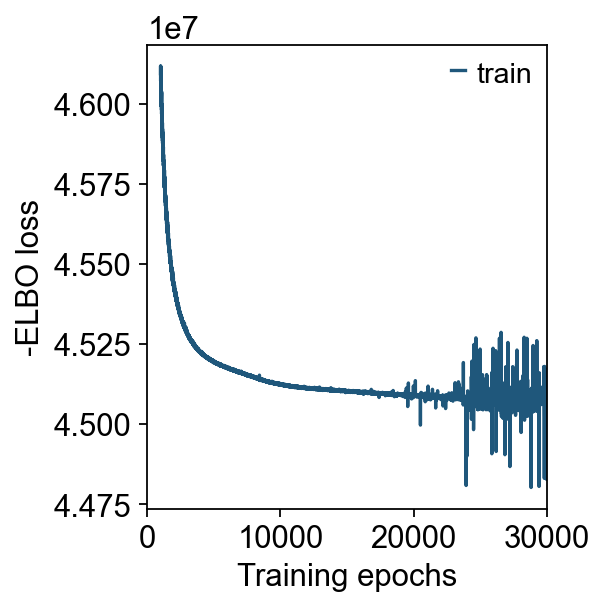
decov_obj.mod_sc.plot_history(20)
ov.plt.show()
decov_obj.mod_sp.plot_history(1000)
Step 4.2 Spatial mapping and saving models (<1 min to save)#
Recommended to save separately:
Parameters/models from reference learning
Parameters/models from spatial mapping This minimizes repeated training costs in future runs.
# Save model
#ov.utils.save(decov_obj.mod_sc,f"result/model/reference_signatures.pkl")
# Save model
ov.utils.save(decov_obj.mod_sp,f"result/model/cell2location_map.pkl")
💾 Save Operation:
   Target path: result/model/reference_signatures.pkl
   Object type: RegressionModel
   Using: pickle
   Pickle failed, switching to: cloudpickle
   ✅ Successfully saved using cloudpickle!
────────────────────────────────────────────────────────────
💾 Save Operation:
   Target path: result/model/cell2location_map.pkl
   Object type: Cell2location
   Using: pickle
   Pickle failed, switching to: cloudpickle
   ✅ Successfully saved using cloudpickle!
────────────────────────────────────────────────────────────
decov_obj.adata_sc.write(f"result/model/cell2location_adata_sc.h5ad")
decov_obj.adata_sp.write(f"result/model/cell2location_adata_sp.h5ad")
Step 4.3 Result object: cell locations (cell2location)#
decov_obj.adata_cell2location
AnnData object with n_obs × n_vars = 4035 × 34
    obs: 'in_tissue', 'array_row', 'array_col', 'sample', '_indices', '_scvi_batch', '_scvi_labels'
    uns: 'spatial', '_scvi_uuid', '_scvi_manager_uuid', 'mod'
    obsm: 'spatial', 'means_cell_abundance_w_sf', 'stds_cell_abundance_w_sf', 'q05_cell_abundance_w_sf', 'q95_cell_abundance_w_sf', 'prop_celltypes'
Step 4.4 Reuse: reload models and perform imputation#
decov_obj=ov.space.Deconvolution(
    adata_sc=ov.read(f"result/model/cell2location_adata_sc.h5ad"),
    adata_sp=ov.read(f"result/model/cell2location_adata_sp.h5ad"),
)
decov_obj.load_cell2location_model(
    mod_sp_path=f"result/model/cell2location_map.pkl"
)
decov_obj.cell2location_inference()
decov_obj.impute(method='cell2location')
decov_obj.adata_sp
📂 Load Operation:
   Source path: result/model/cell2location_map.pkl
   Using: pickle
   ✅ Successfully loaded!
   Loaded object type: Cell2location
────────────────────────────────────────────────────────────
✓ cell2location model is loaded
The cell2location model is saved in self.mod_sc and self.mod_sp
INFO     AnnData object appears to be a copy. Attempting to transfer setup.
✓ cell2location is done
The cell2location result is saved in self.adata_cell2location
✓ cell2location impute is done
Compare with the tangram impute result, cell2location's impute stores in self.adata_sp.layers
AnnData object with n_obs × n_vars = 4035 × 10141
    obs: 'in_tissue', 'array_row', 'array_col', 'sample', '_indices', '_scvi_batch', '_scvi_labels'
    var: 'gene_ids', 'feature_types', 'genome'
    uns: '_scvi_manager_uuid', '_scvi_uuid', 'mod', 'spatial'
    obsm: 'means_cell_abundance_w_sf', 'prop_celltypes', 'q05_cell_abundance_w_sf', 'q95_cell_abundance_w_sf', 'spatial', 'stds_cell_abundance_w_sf'
    layers: 'B_Cycling', 'B_GC_DZ', 'B_GC_LZ', 'B_GC_prePB', 'B_IFN', 'B_activated', 'B_mem', 'B_naive', 'B_plasma', 'B_preGC', 'DC_CCR7+', 'DC_cDC1', 'DC_cDC2', 'DC_pDC', 'Endo', 'FDC', 'ILC', 'Macrophages_M1', 'Macrophages_M2', 'Mast', 'Monocytes', 'NK', 'NKT', 'T_CD4+', 'T_CD4+_TfH', 'T_CD4+_TfH_GC', 'T_CD4+_naive', 'T_CD8+_CD161+', 'T_CD8+_cytotoxic', 'T_CD8+_naive', 'T_TIM3+', 'T_TfR', 'T_Treg', 'VSMC'
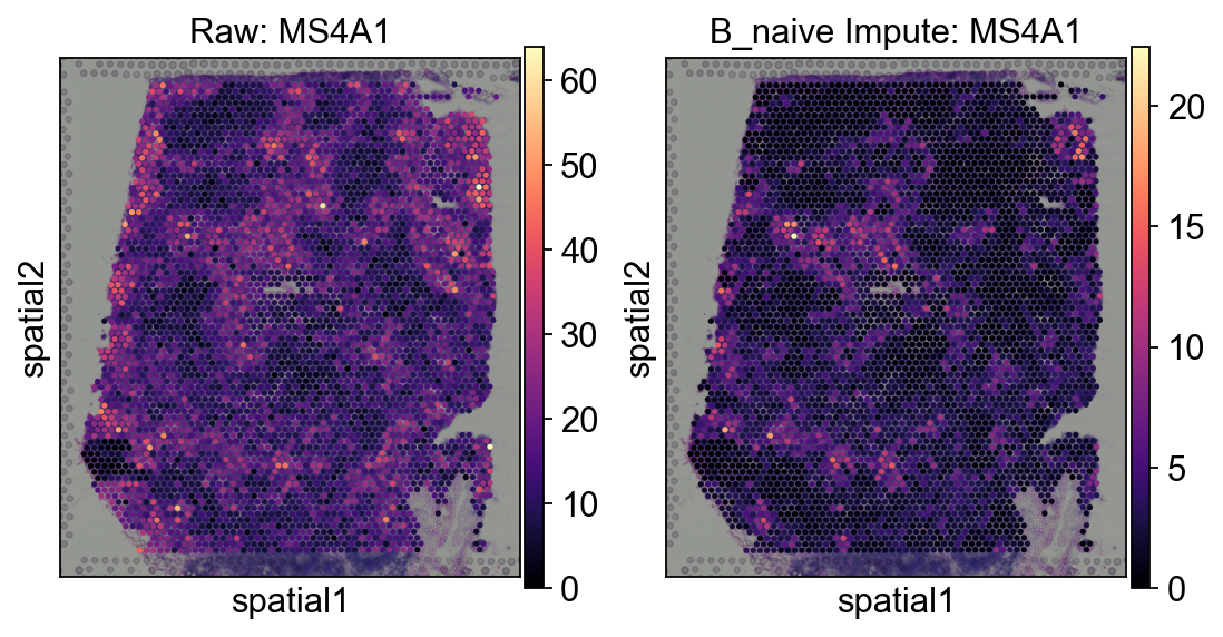
#fig = ov.plt.figure(figsize=(4, 4))
fig, axes = ov.plt.subplots(1,2,figsize=(8, 4))
sc.pl.spatial(
    decov_obj.adata_sp,
    cmap='magma',
    color='MS4A1',
    ncols=4, size=1.3,ax=axes[0],
    img_key='hires',show=False,
)
axes[0].set_title('Raw: MS4A1')

sc.pl.spatial(
    decov_obj.adata_sp,
    layer='B_naive',
    cmap='magma',
    color='MS4A1',
    ncols=4, size=1.3,ax=axes[1],
    img_key='hires',show=False,
)
axes[1].set_title('B_naive Impute: MS4A1')
Text(0.5, 1.0, 'B_naive Impute: MS4A1')
Step 5: Visualization (5–15 min)#
We provide multiple views: single-target spatial heatmaps, multi-target overlays, and local pie charts. Start with global inspection, then zoom into biologically relevant regions for higher-resolution assessment.
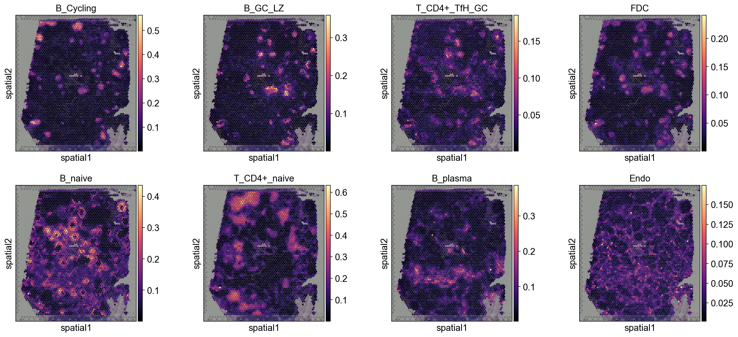
5.1 Spatial value dotplot#
5.1.1 Tangram#
annotation_list=['B_Cycling', 'B_GC_LZ', 'T_CD4+_TfH_GC', 'FDC',
                'B_naive', 'T_CD4+_naive', 'B_plasma', 'Endo']
sc.pl.spatial(
    decov_obj.adata_cell2location,
    cmap='magma',
    # show first 8 cell types
    color=annotation_list,
    ncols=4, size=1.3,
    img_key='hires',
    # limit color scale at 99.2% quantile of cell abundance
    #vmin=0, vmax='p99.2'
)
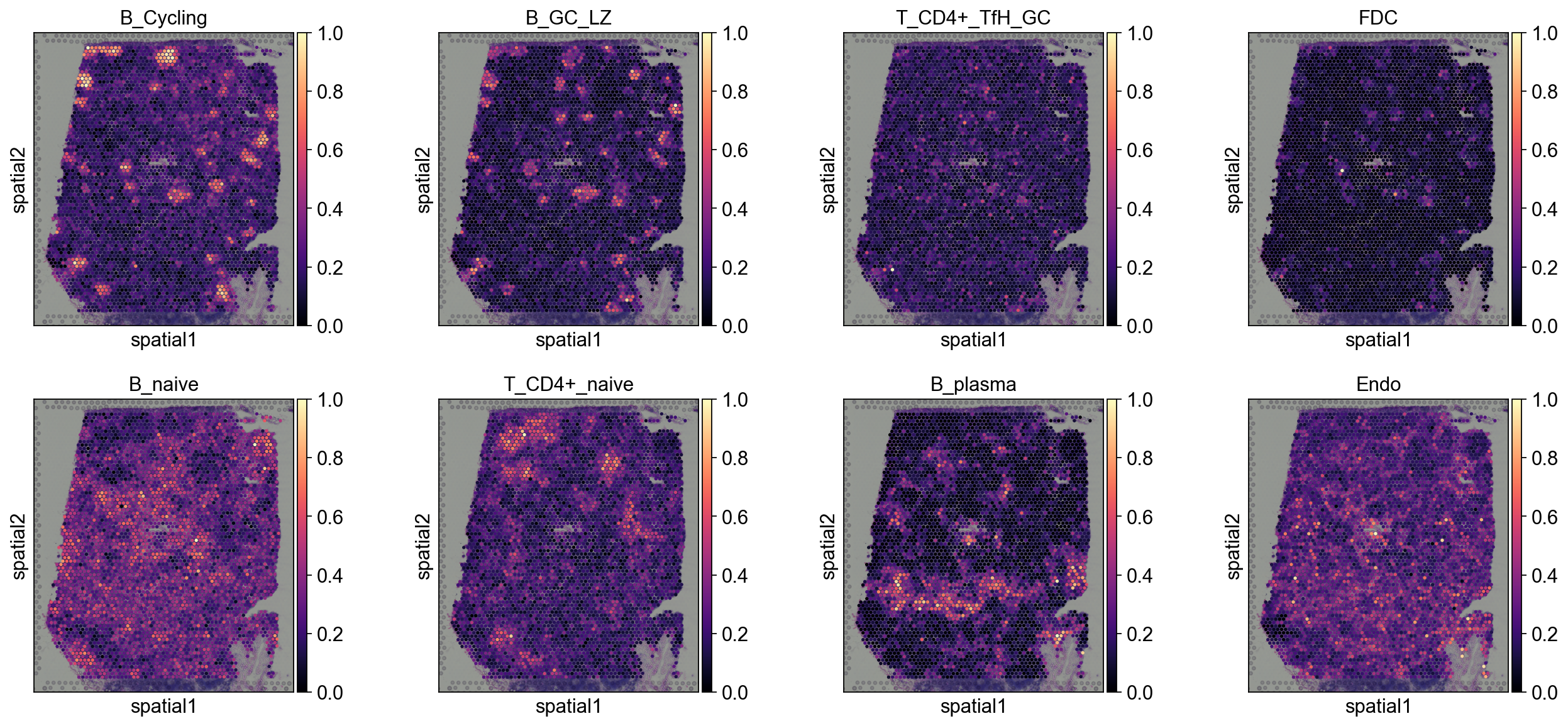
5.1.2 cell2location#
annotation_list=['B_Cycling', 'B_GC_LZ', 'T_CD4+_TfH_GC', 'FDC',
                'B_naive', 'T_CD4+_naive', 'B_plasma', 'Endo']
sc.pl.spatial(
    decov_obj.adata_cell2location,
    cmap='magma',
    # show first 8 cell types
    color=annotation_list,
    ncols=4, size=1.3,
    img_key='hires',
    # limit color scale at 99.2% quantile of cell abundance
    #vmin=0, vmax='p99.2'
)
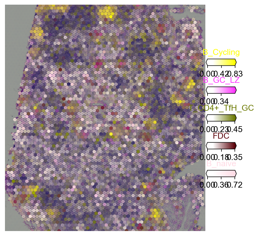
5.2 Multi-target overlay#
color_dict=dict(zip(adata_sc.obs['Subset'].cat.categories,
                   adata_sc.uns['Subset_colors']))
5.2.1 Tangram#
import matplotlib as mpl
clust_labels = annotation_list[:5]
clust_col = ['' + str(i) for i in clust_labels] # in case column names differ from labels

with mpl.rc_context({'figure.figsize': (6, 6),'axes.grid': False}):
    fig = ov.pl.plot_spatial(
        adata=decov_obj.adata_cell2location,
        # labels to show on a plot
        color=clust_col, labels=clust_labels,
        show_img=True,
        # 'fast' (white background) or 'dark_background'
        style='fast',
        # limit color scale at 99.2% quantile of cell abundance
        max_color_quantile=0.992,
        # size of locations (adjust depending on figure size)
        circle_diameter=4,
        reorder_cmap = [#0,
            1,2,3,4,6], #['yellow', 'orange', 'blue', 'green', 'purple', 'grey', 'white'],
        colorbar_position='right',
        palette=color_dict
    )
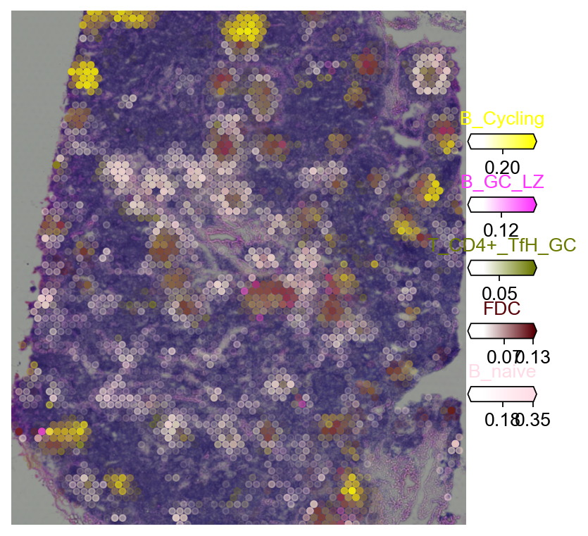
5.2.2 cell2location#
import matplotlib as mpl
clust_labels = annotation_list[:5]
clust_col = ['' + str(i) for i in clust_labels] # in case column names differ from labels

with mpl.rc_context({'figure.figsize': (6, 6),'axes.grid': False}):
    fig = ov.pl.plot_spatial(
        adata=decov_obj.adata_cell2location,
        # labels to show on a plot
        color=clust_col, labels=clust_labels,
        show_img=True,
        # 'fast' (white background) or 'dark_background'
        style='fast',
        # limit color scale at 99.2% quantile of cell abundance
        max_color_quantile=0.992,
        # size of locations (adjust depending on figure size)
        circle_diameter=4,
        reorder_cmap = [#0,
            1,2,3,4,6], #['yellow', 'orange', 'blue', 'green', 'purple', 'grey', 'white'],
        colorbar_position='right',
        palette=color_dict
    )
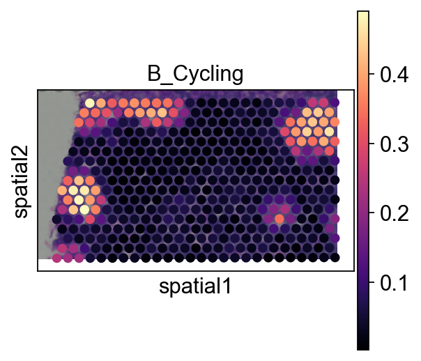
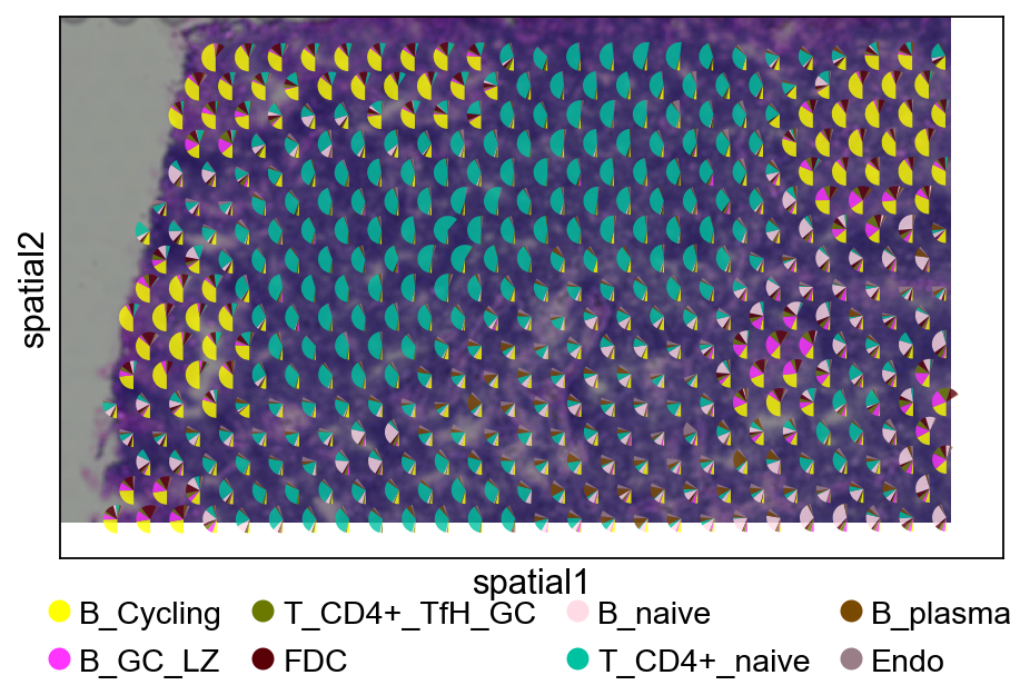
5.3 Pie plot#
We recommend cropping a region of interest before plotting to avoid overly dense pie charts on whole slides.
adata_s = ov.space.crop_space_visium(
    decov_obj.adata_cell2location,
    crop_loc=(0, 0),
    crop_area=(500, 1000),
    library_id=list(decov_obj.adata_cell2location.uns['spatial'].keys())[0] ,
    scale=1
)
Adding image layer `image`
sc.pl.spatial(adata_s, cmap='magma',
                  # show first 8 cell types
                  color=annotation_list[0],
                  ncols=4, size=1.3,
                  img_key='hires',
                  # limit color scale at 99.2% quantile of cell abundance
                  #vmin=0, vmax='p99.2'
                 )
color_dict=dict(zip(adata_sc.obs['Subset'].cat.categories,
                   adata_sc.uns['Subset_colors']))
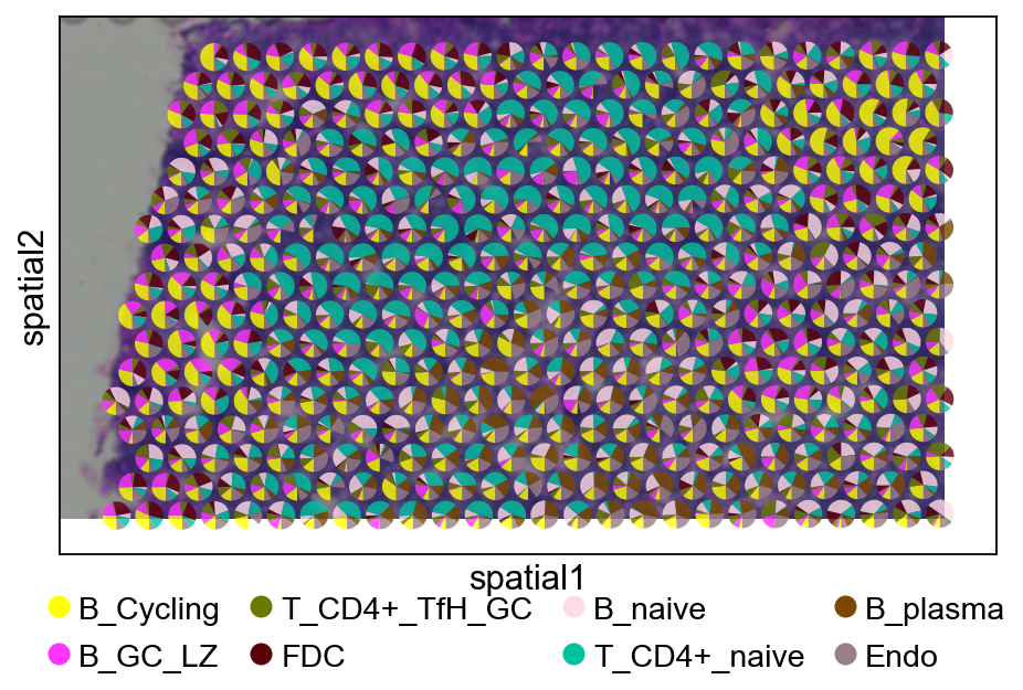
5.3.1 Tangram#
fig, ax = plt.subplots(figsize=(8, 4))
sc.pl.spatial(
    adata_s,
    basis='spatial',
    color=None,
    size=1.3,
    img_key='hires',
    ax=ax,
    show=False
)

ov.pl.add_pie2spatial(
    adata_s,
    img_key='hires',
    cell_type_columns=annotation_list[:],
    ax=ax,
    colors=color_dict,
    pie_radius=10,
    remainder='gap',
    legend_loc=(0.5, -0.25),
    ncols=4,
    alpha=0.8
)

plt.show()
5.3.2 cell2location#
fig, ax = plt.subplots(figsize=(8, 4))
sc.pl.spatial(
    adata_s,
    basis='spatial',
    color=None,
    size=1.3,
    img_key='hires',
    ax=ax,
    show=False
)

ov.pl.add_pie2spatial(
    adata_s,
    img_key='hires',
    cell_type_columns=annotation_list[:],
    ax=ax,
    colors=color_dict,
    pie_radius=10,
    remainder='gap',
    legend_loc=(0.5, -0.25),
    ncols=4,
    alpha=0.8
)

plt.show()
Step 6: Tissue zones via NMF co-localisation (1–3 min)#
Once a deconvolver (Cell2location or Tangram above) has given us
per-spot cell-type abundances, a standard follow-up is to ask
which groups of cell types co-locate? Groups that appear together
repeatedly across the slide are the tissue’s cellular compartments
/ tissue zones (germinal centre, T-cell zone, stromal compartment).
The canonical Cell2location tutorial answers this via a Bayesian
CoLocatedGroupsSklearnNMF (pyro); here we use the lighter-weight
ov.space.nmf_tissue_zones helper that runs scikit-learn NMF on the
cell-abundance matrix. Seconds instead of minutes, same interpretation.
We run this twice — once on Cell2location’s q05_cell_abundance_w_sf
(Step 6A), once on Tangram’s tangram_ct_pred (Step 6B) — to show the
same analysis works on either backend.
Step 6.0 Style setup#
Make sure the omicverse plot style is active so this section’s figures match the rest of the tutorial.
ov.plot_set()
🔬 Starting plot initialization...
🧬 Detecting GPU devices…
✅ NVIDIA CUDA GPUs detected: 1
    • [CUDA 0] NVIDIA H100 80GB HBM3
      Memory: 79.1 GB | Compute: 9.0

   ____            _     _    __
  / __ \____ ___  (_)___| |  / /__  _____________
 / / / / __ `__ \/ / ___/ | / / _ \/ ___/ ___/ _ \
/ /_/ / / / / / / / /__ | |/ /  __/ /  (__  )  __/
\____/_/ /_/ /_/_/\___/ |___/\___/_/  /____/\___/

🔖 Version: 2.1.2rc1   📚 Tutorials: https://omicverse.readthedocs.io/
✅ plot_set complete.
Step 6A.1 Run NMF on Cell2location abundances#
tz_c2l = ov.space.nmf_tissue_zones(
    decov_obj.adata_sp,
    obsm_key='q05_cell_abundance_w_sf',
    n_factors=10,
    top_k=5,
    seed=0,
)
print(f'reconstruction error: {tz_c2l.reconstruction_err:.2f}')
print(f'spot activations in obsm["X_tissue_zones"], '
      f'shape={decov_obj.adata_sp.obsm["X_tissue_zones"].shape}')
reconstruction error: 80.74
spot activations in obsm["X_tissue_zones"], shape=(4035, 10)
Step 6A.2 Top cell types per zone (Cell2location)#
for zone, top_cts in tz_c2l.factor_top_cell_types.items():
    print(f'{zone}: {", ".join(top_cts)}')
zone_1: B_mem, B_naive, DC_cDC1, T_CD4+_naive, FDC
zone_2: T_CD4+_naive, T_CD8+_naive, T_TfR, T_Treg, DC_CCR7+
zone_3: B_Cycling, B_GC_DZ, FDC, DC_cDC1, Macrophages_M1
zone_4: B_preGC, DC_cDC1, B_Cycling, T_CD4+_naive, T_TIM3+
zone_5: T_TIM3+, NK, B_preGC, DC_pDC, T_TfR
zone_6: B_IFN, T_TIM3+, FDC, B_plasma, T_TfR
zone_7: B_naive, B_mem, B_activated, T_CD4+_TfH_GC, B_preGC
zone_8: Macrophages_M1, Endo, DC_cDC2, VSMC, Monocytes
zone_9: B_plasma, B_activated, Macrophages_M2, B_naive, VSMC
zone_10: B_GC_LZ, T_CD4+_TfH_GC, FDC, Macrophages_M1, B_activated
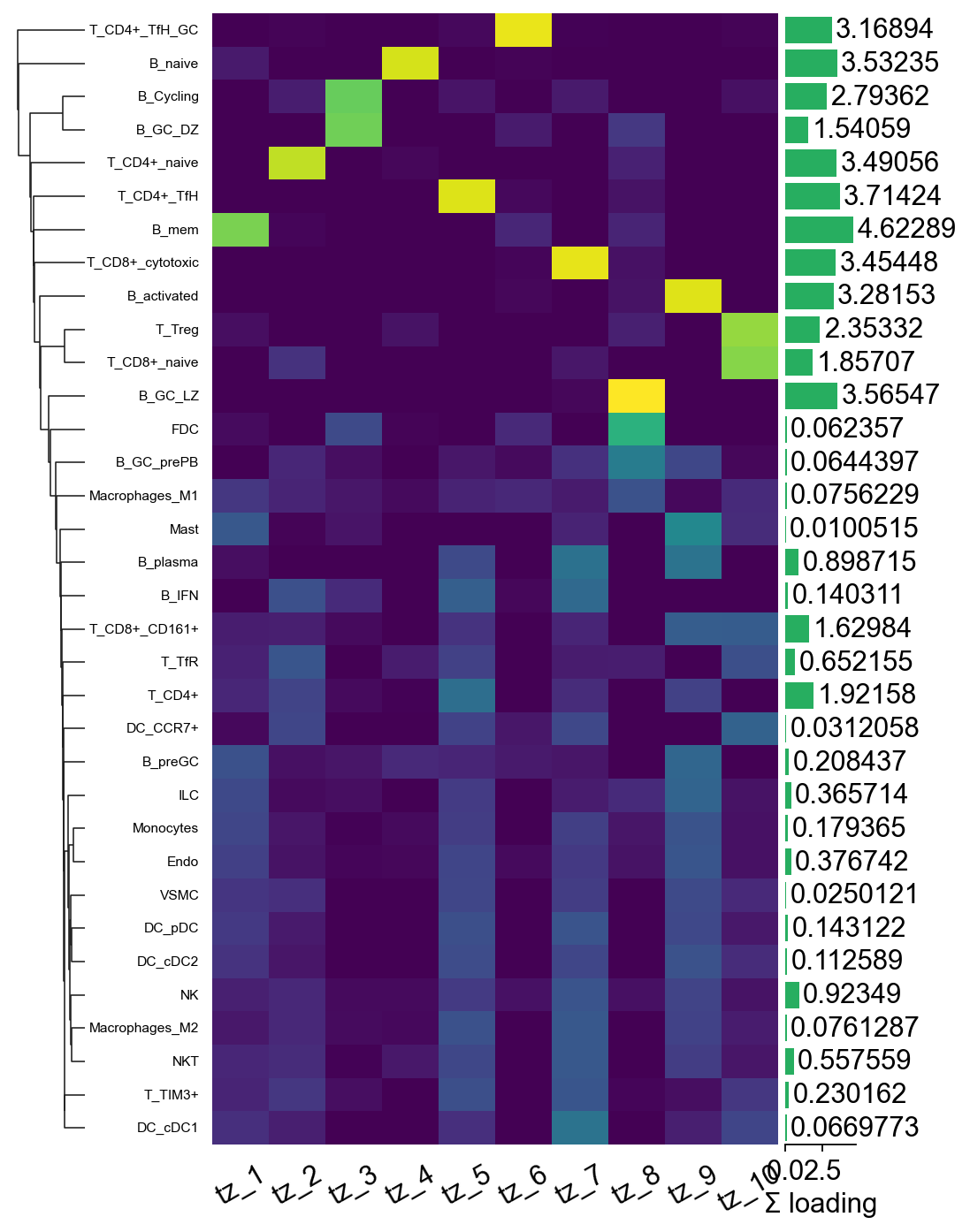
Step 6A.3 Factor-loadings heatmap via marsilea#
marsilea gives a much nicer composable heatmap than raw
matplotlib: auto-clustering on both axes, side annotations for the
per-factor “top cell type” label and the per-cell-type total
loading, and a built-in legend. We row-normalise the loadings so
the colour scale reflects relative importance rather than
absolute magnitude.
import marsilea as ma
import marsilea.plotter as mp
import numpy as np

mat_n = tz_c2l.factor_loadings.div(tz_c2l.factor_loadings.sum(axis=1) + 1e-9, axis=0)
row_totals = tz_c2l.factor_loadings.sum(axis=1).values

h = ma.Heatmap(
    mat_n.values, cmap='viridis',
    width=4, height=8,                 # taller to fit 34 cell types
    cbar_kws=dict(title='normalised\nloading'),
)
h.add_bottom(mp.Labels(mat_n.columns.tolist(), rotation=30), pad=0.1)
h.add_left(mp.Labels(mat_n.index.tolist(), align='right',
                     fontsize=7), pad=0.08)
h.add_right(mp.Numbers(row_totals, color='#2980b9',
                        label='Σ loading'), size=0.5, pad=0.05)
h.add_dendrogram('left')
h.render()
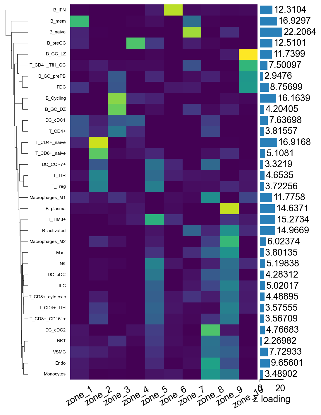
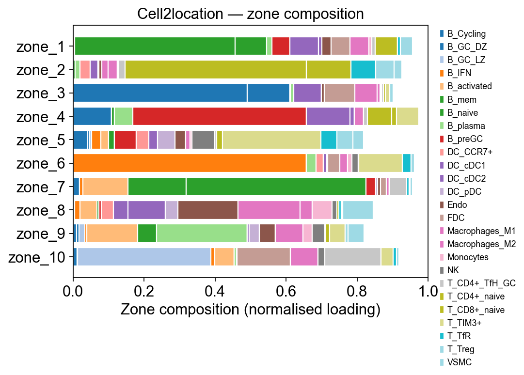
Step 6A.4 Zone composition — per-zone cell-type breakdown#
The heatmap shows where the signal lives but can’t be read by row sum. A stacked horizontal bar per zone makes the composition obvious: each zone is one bar, each coloured segment is a cell type, width = its normalised contribution to that zone.
import matplotlib.pyplot as plt
import numpy as np

# Build a zone × cell-type normalised composition matrix limited to
# the top-K contributors across *any* zone. This keeps the legend
# manageable (~15 cell types instead of 34).
loadings = tz_c2l.factor_loadings          # (n_celltypes, n_factors)
per_zone = loadings.div(loadings.sum(axis=0) + 1e-9, axis=1)
# Contributing cell types: anyone who tops 5 in some zone OR
# whose max loading exceeds 0.05
contrib = set()
for f in per_zone.columns:
    contrib.update(per_zone[f].sort_values(ascending=False).head(5).index)
contrib = sorted(contrib)
print(f'{len(contrib)} distinct cell types across all zones top-5')

comp = per_zone.loc[contrib]                 # (n_contrib, n_factors)

fig, ax = plt.subplots(figsize=(7, 0.35 * comp.shape[1] + 1.2))
cmap = plt.get_cmap('tab20', len(contrib))
bottom = np.zeros(comp.shape[1])
zones = comp.columns.tolist()
for i, ct in enumerate(comp.index):
    vals = comp.loc[ct].values
    ax.barh(zones, vals, left=bottom, color=cmap(i),
            edgecolor='white', label=ct)
    bottom += vals
ax.set_xlabel('Zone composition (normalised loading)')
ax.set_ylabel('')
ax.set_xlim(0, 1.0)
ax.invert_yaxis()
ax.legend(bbox_to_anchor=(1.02, 1.0), loc='upper left',
          frameon=False, fontsize=8)
ax.set_title('Cell2location — zone composition')
fig.tight_layout()
plt.show()
26 distinct cell types across all zones top-5
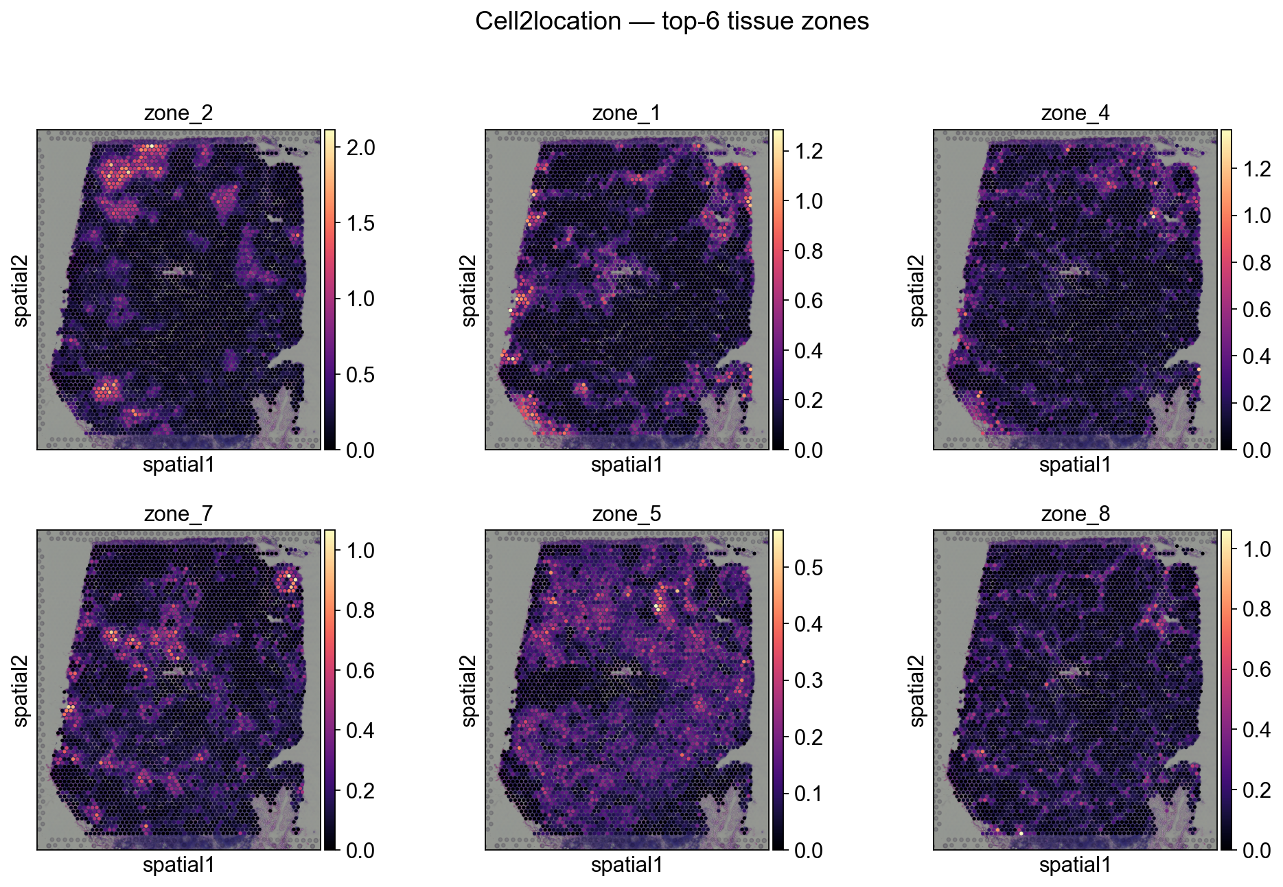
Step 6A.5 Plot tissue zones in the slide (Cell2location)#
# Expose per-factor activations on .obs for scanpy spatial plotting
for i, zn in enumerate(tz_c2l.factor_names):
    decov_obj.adata_sp.obs[zn] = decov_obj.adata_sp.obsm['X_tissue_zones'][:, i]

# Top-6 zones by total activation
totals = tz_c2l.spot_activations.sum(axis=0).sort_values(ascending=False)
top_zones = totals.head(6).index.tolist()
print('Top zones by total activation:', top_zones)

sc.pl.spatial(
    decov_obj.adata_sp,
    color=top_zones, ncols=3, size=1.3, img_key='hires',
    cmap='magma', show=False,
)
plt.suptitle('Cell2location — top-6 tissue zones', y=1.02)
plt.show()
Top zones by total activation: ['zone_2', 'zone_1', 'zone_4', 'zone_7', 'zone_5', 'zone_8']
Step 6B — Same NMF on Tangram output#
Tangram writes its per-cell-type prediction matrix to
adata.obsm['tangram_ct_pred'] (spots × cell types). The API is
identical — just change obsm_key= and pick a fresh obsm key for
the result.
Caveat: Tangram’s matrix stores mapping probabilities, not
absolute abundances. Different spots have very different total
signal, so a raw NMF tends to put all that total-signal variance
into the first factor. Pass normalize='rows' (new in v0.x) to
feed NMF the row-stochastic composition instead — this is the
apples-to-apples input for a Tangram-specific tissue-zone
decomposition. For Cell2location’s q05_cell_abundance_w_sf
(Step 6A) we leave it raw because the absolute-abundance scale
is biologically meaningful.
# Load the Tangram-decomposed slide (saved in Step 3.3)
import anndata as ad
_tangram_path = 'result/model/tangram_adata_sp.h5ad'
try:
    adata_sp_tangram = ad.read_h5ad(_tangram_path)
except FileNotFoundError:
    adata_sp_tangram = decov_obj.adata_sp  # fallback to current slide
    print('Tangram cache not found — reusing the current adata_sp')

tz_tan = ov.space.nmf_tissue_zones(
    adata_sp_tangram,
    obsm_key='tangram_ct_pred',
    n_factors=10,
    normalize='rows',  # compositional scale — see Caveat
    top_k=5,
    obsm_added='X_tissue_zones_tangram',
    factor_prefix='tz',
    seed=0,
)
print(f'reconstruction error: {tz_tan.reconstruction_err:.2f}')
for zone, top_cts in tz_tan.factor_top_cell_types.items():
    print(f'{zone}: {", ".join(top_cts[:3])}…')
reconstruction error: 3.77
tz_1: B_mem, B_naive, T_CD4+…
tz_2: T_CD4+_naive, T_CD4+, T_CD8+_naive…
tz_3: B_Cycling, B_GC_DZ, T_CD4+…
tz_4: B_naive, T_Treg, T_CD4+_naive…
tz_5: T_CD4+_TfH, T_CD4+, T_CD8+_CD161+…
tz_6: T_CD4+_TfH_GC, B_mem, B_GC_DZ…
tz_7: T_CD8+_cytotoxic, B_plasma, NK…
tz_8: B_GC_LZ, B_mem, T_CD4+_naive…
tz_9: B_activated, T_CD8+_CD161+, T_CD4+…
tz_10: T_Treg, T_CD8+_naive, T_CD8+_CD161+…
Step 6B.2 Factor-loadings heatmap (Tangram)#
import marsilea as ma
import marsilea.plotter as mp
import numpy as np

mat_n = tz_tan.factor_loadings.div(tz_tan.factor_loadings.sum(axis=1) + 1e-9, axis=0)
row_totals = tz_tan.factor_loadings.sum(axis=1).values

h = ma.Heatmap(
    mat_n.values, cmap='viridis',
    width=4, height=8,                 # taller to fit 34 cell types
    cbar_kws=dict(title='normalised\nloading'),
)
h.add_bottom(mp.Labels(mat_n.columns.tolist(), rotation=30), pad=0.1)
h.add_left(mp.Labels(mat_n.index.tolist(), align='right',
                     fontsize=7), pad=0.08)
h.add_right(mp.Numbers(row_totals, color='#27ae60',
                        label='Σ loading'), size=0.5, pad=0.05)
h.add_dendrogram('left')
h.render()
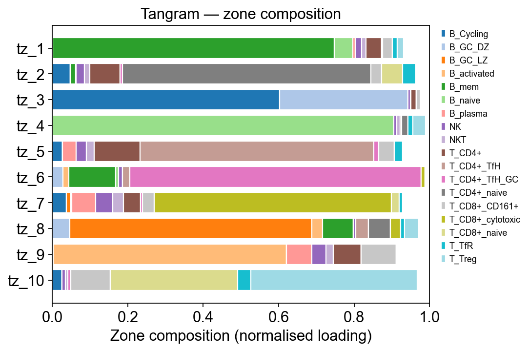
Step 6B.3 Zone composition — per-zone cell-type breakdown#
The heatmap shows where the signal lives but can’t be read by row sum. A stacked horizontal bar per zone makes the composition obvious: each zone is one bar, each coloured segment is a cell type, width = its normalised contribution to that zone.
import matplotlib.pyplot as plt
import numpy as np

# Build a zone × cell-type normalised composition matrix limited to
# the top-K contributors across *any* zone. This keeps the legend
# manageable (~15 cell types instead of 34).
loadings = tz_tan.factor_loadings          # (n_celltypes, n_factors)
per_zone = loadings.div(loadings.sum(axis=0) + 1e-9, axis=1)
# Contributing cell types: anyone who tops 5 in some zone OR
# whose max loading exceeds 0.05
contrib = set()
for f in per_zone.columns:
    contrib.update(per_zone[f].sort_values(ascending=False).head(5).index)
contrib = sorted(contrib)
print(f'{len(contrib)} distinct cell types across all zones top-5')

comp = per_zone.loc[contrib]                 # (n_contrib, n_factors)

fig, ax = plt.subplots(figsize=(7, 0.35 * comp.shape[1] + 1.2))
cmap = plt.get_cmap('tab20', len(contrib))
bottom = np.zeros(comp.shape[1])
zones = comp.columns.tolist()
for i, ct in enumerate(comp.index):
    vals = comp.loc[ct].values
    ax.barh(zones, vals, left=bottom, color=cmap(i),
            edgecolor='white', label=ct)
    bottom += vals
ax.set_xlabel('Zone composition (normalised loading)')
ax.set_ylabel('')
ax.set_xlim(0, 1.0)
ax.invert_yaxis()
ax.legend(bbox_to_anchor=(1.02, 1.0), loc='upper left',
          frameon=False, fontsize=8)
ax.set_title('Tangram — zone composition')
fig.tight_layout()
plt.show()
18 distinct cell types across all zones top-5
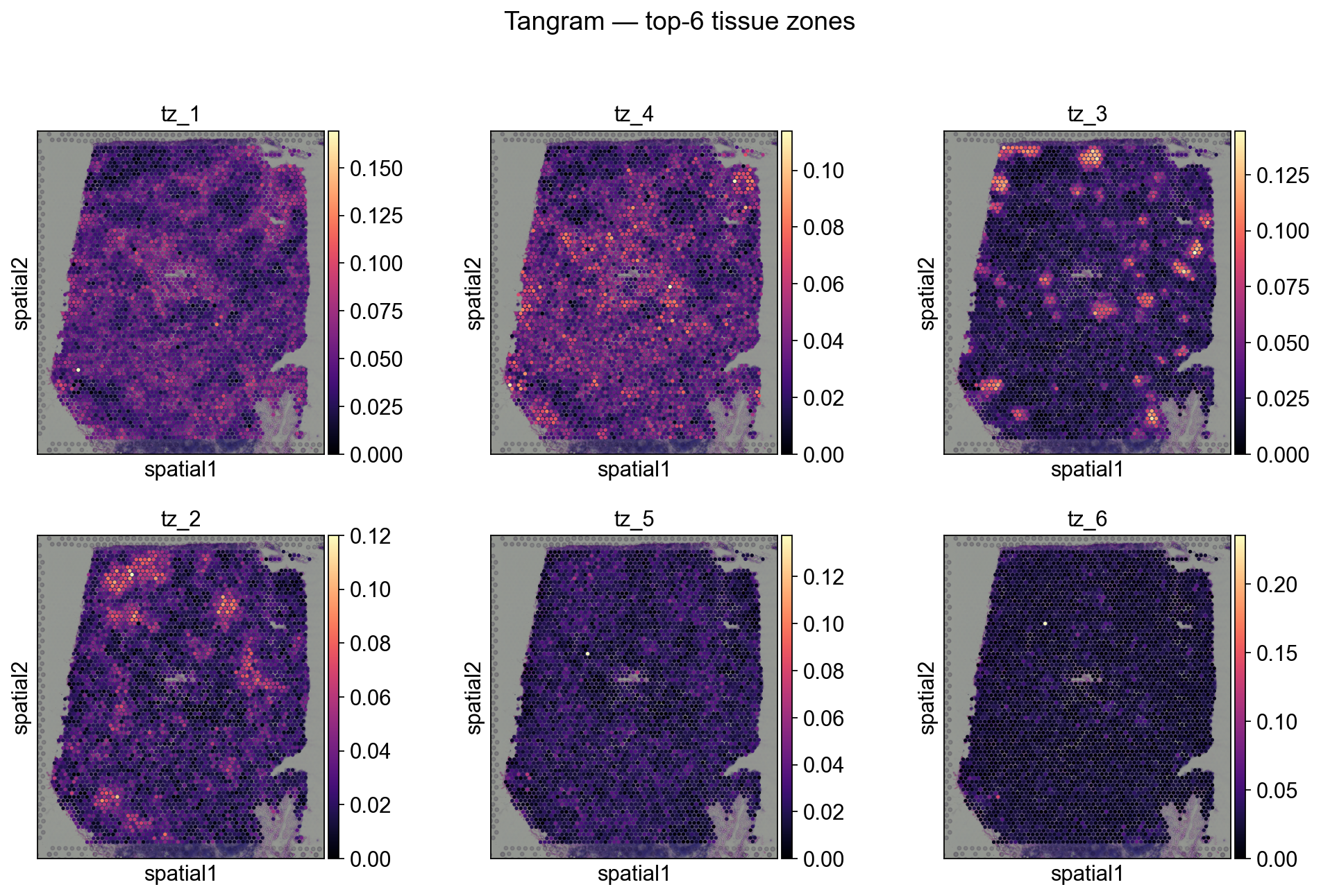
Step 6B.4 Zones in the slide (Tangram)#
for i, zn in enumerate(tz_tan.factor_names):
    adata_sp_tangram.obs[zn] = adata_sp_tangram.obsm['X_tissue_zones_tangram'][:, i]

totals_t = tz_tan.spot_activations.sum(axis=0).sort_values(ascending=False)
top_zones_t = totals_t.head(6).index.tolist()
print('Top zones by total activation:', top_zones_t)

sc.pl.spatial(
    adata_sp_tangram,
    color=top_zones_t, ncols=3, size=1.3, img_key='hires',
    cmap='magma', show=False,
)
plt.suptitle('Tangram — top-6 tissue zones', y=1.02)
plt.show()
Top zones by total activation: ['tz_1', 'tz_4', 'tz_3', 'tz_2', 'tz_5', 'tz_6']
Step 6.5 Reusable helper#
The full pipeline for either backend is two calls:
decov_obj.deconvolution(method='cell2location')   # or method='Tangram'
tz = ov.space.nmf_tissue_zones(
    decov_obj.adata_sp,
    obsm_key='q05_cell_abundance_w_sf',             # or 'tangram_ct_pred'
    n_factors=10,
)
The full Bayesian equivalent (from the Cell2location paper) is at
ov.external.space.cell2location.run_colocation — pyro-backed,
~10 min per slide.
Extensions and Further Reading#
cell2location official tutorials and docs: https://cell2location.readthedocs.io/en/latest/notebooks/cell2location_tutorial.html
Tangram paper and documentation: consult official resources for advanced parameters and updates.
Reproducibility tip: record
omicverseand dependency versions in your project for consistent results across the team.
from omicverse.external.space.cell2location.models import Cell2location, RegressionModel
from omicverse.external.space.cell2location.plt import plot_spatial
from omicverse.external.space.cell2location.utils import select_slide
from omicverse.external.space.cell2location.utils.filtering import filter_genes
Citations and Acknowledgements#
Please cite:
OmicVerse toolkit (this notebook’s implementation)
Tangram: original publication and software
cell2location: original publication and software
The datasets used (scRNA-seq reference and spatial transcriptomics)
We thank the original tool authors and dataset providers for making their resources available to the community.
import tangram as tg
Troubleshooting#
Gene ID mismatch:
Symptom: many NaNs or empty outputs; very few overlapping genes.
Fix: harmonize gene IDs between scRNA-seq and spatial data (ENSEMBL/symbols), drop non-overlapping genes and log counts.
Reference coverage insufficient:
Symptom: expected cell types missing in known tissue regions.
Fix: augment the scRNA-seq reference with tissue/age/pathology-matched data; integrate multiple sources and correct batch effects.
Hyperparameters:
Tangram: pay attention to regularization and gene selection; small grid search can help.
cell2location: prefer GPU; adjust training epochs/priors to dataset size; monitor convergence diagnostics.
Reproducibility:
Fix random seeds and package versions; save models and key intermediate artifacts; record environment details at the top of the notebook.