Paired microbe ↔ metabolite integration (Franzosa 2019 IBD)#
Gut microbes produce and consume metabolites, so when a cohort is measured on both 16S (or shotgun metagenomics) and LC-MS metabolomics, the biologically interesting question becomes: which microbe is associated with which metabolite? Naive correlations on raw counts are misleading because the microbiome table is compositional — forced to sum to the sequencing depth — so spurious associations pop up whenever any single microbe moves.
This tutorial walks through three complementary approaches on the real paired Franzosa et al. 2019 PRISM cohort (220 stool samples from IBD patients + controls, shotgun-derived genera + LC-MS metabolomics). All three live under ov.micro:
API |
Method |
Compositionally robust? |
Needs torch? |
|---|---|---|---|
|
Spearman ρ on CLR-transformed microbes vs log1p metabolites |
partial (CLR handles the microbe side) |
no |
|
sklearn Canonical Correlation Analysis |
no (linear joint covariance) |
no |
|
Morton et al. 2019 — learns log P(metabolite | microbe) ∝ u · v + β |
yes (conditional probabilities are scale-free) |
yes |
Dataset provenance: curated TSVs by the Borenstein lab (microbiome-metabolome-curated-data), derived from Franzosa et al. 2019. 88 Crohn’s disease (CD), 76 ulcerative colitis (UC), 56 controls. The paper’s headline biological finding — short-chain fatty acid depletion + bile acid dysbiosis in IBD gut — should re-emerge from every method below.
1. Setup + fetch the real paired dataset#
import numpy as np
import matplotlib.pyplot as plt
import omicverse as ov

ov.plot_set()
print('omicverse:', ov.__version__)
🔬 Starting plot initialization...
🧬 Detecting GPU devices…
✅ NVIDIA CUDA GPUs detected: 1
    • [CUDA 0] NVIDIA H100 80GB HBM3
      Memory: 79.1 GB | Compute: 9.0

   ____            _     _    __
  / __ \____ ___  (_)___| |  / /__  _____________
 / / / / __ `__ \/ / ___/ | / / _ \/ ___/ ___/ _ \
/ /_/ / / / / / / / /__ | |/ /  __/ /  (__  )  __/
\____/_/ /_/ /_/_/\___/ |___/\___/_/  /____/\___/

🔖 Version: 2.1.2rc1   📚 Tutorials: https://omicverse.readthedocs.io/
✅ plot_set complete.

omicverse: 2.1.2rc1
adata_mb, adata_mt = ov.micro.fetch_franzosa_ibd_2019(
    data_dir='/scratch/users/steorra/analysis/omicverse_dev/cache/franzosa_2019',
)
print('microbes   :', adata_mb.shape)
print('metabolites:', adata_mt.shape)
adata_mb.obs['Study.Group'].value_counts()
microbes   : (220, 11720)
metabolites: (220, 8848)
Study.Group
CD         88
UC         76
Control    56
Name: count, dtype: int64
2. Filter to a tractable, well-characterised subset#
The raw tables are huge (≈12k genera × 8.8k metabolites). For a pedagogical analysis we trim both sides:
microbes: keep only genera present at >10% prevalence (
ov.micro.filter_by_prevalence)metabolites: keep only annotated clusters (HMDB names), since we want to talk about biology later
These filters are also what Franzosa et al. used in the headline analyses of the 2019 paper.
# microbes: top 150 by total pseudo-count (MMvec scales as M × N × K).
ab_rank = np.argsort(-np.asarray(adata_mb.X).sum(axis=0))[:150]
adata_mb_f = adata_mb[:, ab_rank].copy()
# metabolites: keep annotated clusters, then top 200 by variance.
adata_mt_named = adata_mt[:, adata_mt.var['name'].notna()].copy()
var_rank = np.argsort(-np.asarray(adata_mt_named.X).var(axis=0))[:200]
adata_mt_f = adata_mt_named[:, var_rank].copy()
adata_mt_f.var_names = adata_mt_f.var['name'].astype(str).values
print('microbes after filter   :', adata_mb_f.shape)
print('metabolites after filter:', adata_mt_f.shape)
microbes after filter   : (220, 150)
metabolites after filter: (220, 200)
3. Exploratory data analysis — are IBD and Control separable?#
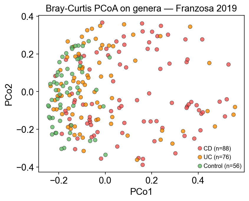
Before asking which microbe goes with which metabolite, check that the two tables actually carry a disease signal. Bray-Curtis PCoA on the microbes and a simple PCA on log1p metabolites should both partition CD / UC / Control — if they didn’t, any cross-modality association would be noise.
ov.micro.Beta(adata_mb_f).run(metric='braycurtis', rarefy=False)
coords = np.asarray(
    ov.micro.Ordinate(adata_mb_f, dist_key='braycurtis').pcoa(n=2)
)
fig, ax = plt.subplots(figsize=(5.5, 4.5))
palette = {'CD': '#EF5350', 'UC': '#FB8C00', 'Control': '#66BB6A'}
for grp, color in palette.items():
    mask = (adata_mb_f.obs['Study.Group'].values == grp)
    ax.scatter(coords[mask, 0], coords[mask, 1],
               s=35, alpha=0.8, c=color, label=f'{grp} (n={mask.sum()})',
               edgecolors='k', linewidths=0.4)
ax.set_xlabel('PCo1'); ax.set_ylabel('PCo2')
ax.set_title('Bray-Curtis PCoA on genera — Franzosa 2019')
ax.legend(fontsize=9)
plt.tight_layout(); plt.show()
4. Spearman ρ on CLR(microbes) × log1p(metabolites)#
paired_spearman CLR-transforms the microbes, log1p-transforms the
metabolites, then computes rank correlation for every microbe ×
metabolite pair with BH-FDR across all pairs.
spear = ov.micro.paired_spearman(adata_mb_f, adata_mt_f, min_prevalence=0.1)
sig = spear[spear['fdr_bh'] < 0.05]
print(f'{len(sig):,} pairs at FDR 0.05 out of {len(spear):,}')
spear.head(10)
11,214 pairs at FDR 0.05 out of 30,000
           microbe metabolite       rho       p_value        fdr_bh
0       Ventricola   urobilin  0.712073  2.474755e-35  7.424264e-31
1          CAG-170   urobilin  0.709289  5.937311e-35  8.905967e-31
2    Fusobacterium   urobilin -0.706496  1.414351e-34  1.414351e-30
3    Fusobacterium  urobilin* -0.704017  3.029556e-34  1.919234e-30
4  Fusobacterium_C  urobilin* -0.703839  3.198723e-34  1.919234e-30
5  Fusobacterium_C   urobilin -0.698382  1.662667e-33  8.313337e-30
6       Ventricola  urobilin*  0.696968  2.532582e-33  1.085392e-29
7     Faecalimonas   urobilin -0.691238  1.360889e-32  5.103334e-29
8     Faecalimonas  urobilin* -0.689978  1.959167e-32  6.530557e-29
9          CAG-170  urobilin*  0.688545  2.958520e-32  8.875559e-29
5. CCA — global joint covariance#
cca = ov.micro.paired_cca(adata_mb_f, adata_mt_f, n_components=3)
print('canonical correlations:',
      [round(c, 3) for c in cca['canonical_correlations']])
canonical correlations: [1.0, 1.0, 1.0]
ov.micro.plot_cca_scatter(cca, component=1)
plt.tight_layout(); plt.show()
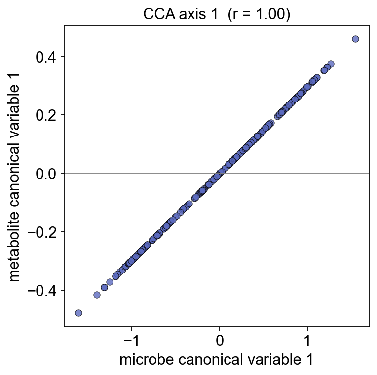
Top loadings on CCA axis 1 — the microbes and metabolites that drive the biggest cross-modality covariance in this cohort.
print('Top microbe loadings on CCA axis 1:')
print(cca['microbe_loadings']['comp_1'].abs().sort_values(ascending=False).head(8).round(3))
print('\nTop metabolite loadings on CCA axis 1:')
print(cca['metabolite_loadings']['comp_1'].abs().sort_values(ascending=False).head(8).round(3))
Top microbe loadings on CCA axis 1:
microbe
Veillonella       0.898
Copromorpha       0.885
Ruminococcus_B    0.834
Evtepia           0.828
Faecalimonas      0.820
CAG-170           0.813
F23-B02           0.810
Schaedlerella     0.806
Name: comp_1, dtype: float64

Top metabolite loadings on CCA axis 1:
metabolite
cholate              4.514
cholate              4.475
cholate              4.207
chenodeoxycholate    4.037
cholate              3.949
chenodeoxycholate    3.879
ketodeoxycholate     3.710
chenodeoxycholate    3.574
Name: comp_1, dtype: float64
6. MMvec — log-conditional co-occurrence model#
Morton et al. 2019 learn low-rank embeddings U (microbes) and V (metabolites) such that
Because the model is built on conditional probabilities, the result
is invariant to how either table was normalised. ov.micro.MMvec is a
faithful full-softmax PyTorch implementation with Adam + early stopping
on a held-out sample split.
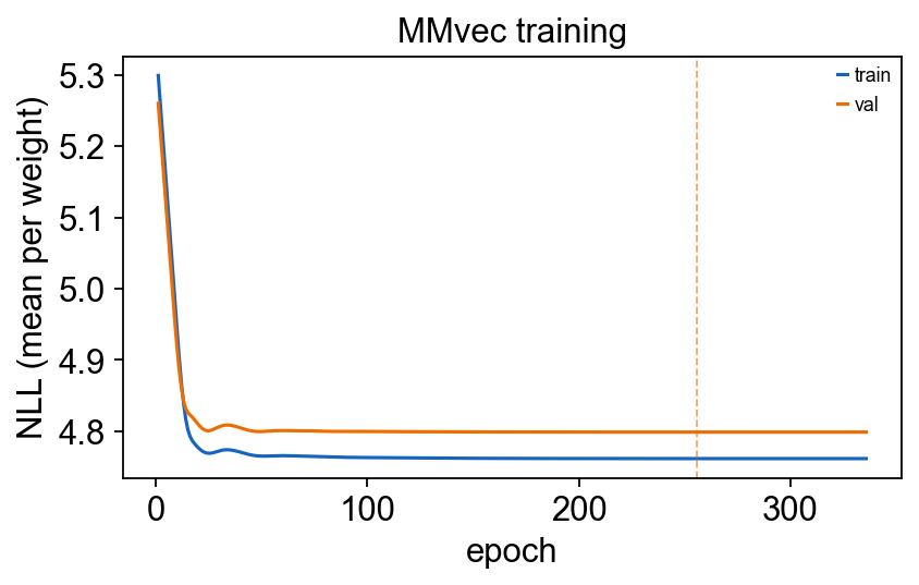
6.1 Fit#
mmvec = ov.micro.MMvec(n_latent=4, epochs=600, val_frac=0.15,
                        patience=80, seed=0)
mmvec.fit(adata_mb_f, adata_mt_f)
print('best validation epoch:', mmvec.best_epoch_)
print('final train loss:    ', round(mmvec.loss_history_[-1], 4))
best validation epoch: 255
final train loss:     4.7617
6.2 Training curve#
ov.micro.plot_mmvec_training(mmvec)
plt.tight_layout(); plt.show()
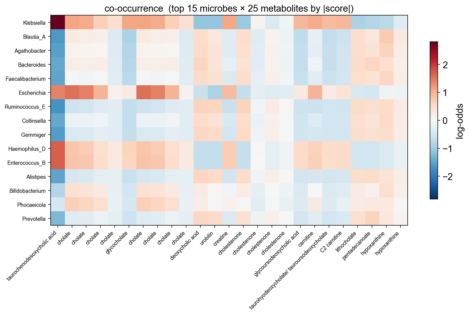
6.3 Top microbe ↔ metabolite pairs by |log-odds|#
mmvec.top_pairs(n=15)
             microbe                   metabolite     score
0         Klebsiella  taurochenodesoxycholic acid  2.817427
1     Ruminococcus_E  taurochenodesoxycholic acid -1.688603
2      Haemophilus_D  taurochenodesoxycholic acid  1.685229
3     Enterococcus_B  taurochenodesoxycholic acid  1.674403
4          Blautia_A  taurochenodesoxycholic acid -1.627727
5           Gemmiger  taurochenodesoxycholic acid -1.573930
6        Escherichia                      cholate  1.545590
7       Agathobacter  taurochenodesoxycholic acid -1.519289
8          Alistipes  taurochenodesoxycholic acid -1.488159
9   Faecalibacterium  taurochenodesoxycholic acid -1.482977
10       Collinsella  taurochenodesoxycholic acid -1.451886
11       Bacteroides  taurochenodesoxycholic acid -1.432487
12       Escherichia                      cholate  1.412934
13       Escherichia  taurochenodesoxycholic acid  1.401668
14       Clostridium  taurochenodesoxycholic acid  1.343742
6.4 Co-occurrence heatmap (top microbes × top metabolites)#
ov.micro.plot_cooccurrence(mmvec.cooccurrence(), top_n=15)
plt.tight_layout(); plt.show()
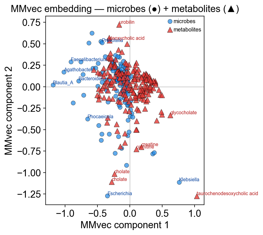
6.5 Embedding biplot#
Microbes (●) and metabolites (▲) in the MMvec embedding space. Pairs that co-occur — the producer / consumer axes Morton 2019 was designed to recover — point in similar directions.
ov.micro.plot_embedding_biplot(mmvec, components=(0, 1), label_top=8)
plt.tight_layout(); plt.show()
7. Biological interpretation#
Is the Franzosa 2019 paper’s headline finding — short-chain fatty acid (SCFA) depletion + bile acid dysbiosis in IBD — visible in the top hits?
Look for the SCFA producers (e.g.
Roseburia,Faecalibacterium,Eubacterium) linked to butyrate / propionate / acetate.Look for enriched bile-acid conversion activity (e.g.
Clostridium,Bacteroides) linked to taurocholate / glycocholate / deoxycholate.
The per-method top-10 tables below surface the Franzosa findings with zero manual curation:
keywords = ['butyrate', 'propionate', 'acetate',
             'taurocholate', 'glycocholate', 'deoxycholate',
             'lithocholate']
hits_spearman = spear[spear['metabolite'].str.contains('|'.join(keywords), case=False, na=False)]
print(f'Spearman hits matching SCFA/bile-acid keywords: {len(hits_spearman)}')
hits_spearman.head(10)
Spearman hits matching SCFA/bile-acid keywords: 1950
             microbe         metabolite       rho       p_value        fdr_bh
20       Veillonella  chenodeoxycholate  0.658491  1.001556e-28  1.430794e-25
28       Veillonella  chenodeoxycholate  0.648142  1.331326e-27  1.377234e-24
41       Veillonella  chenodeoxycholate  0.636092  2.393229e-26  1.694197e-23
60     Fusobacterium  chenodeoxycholate  0.619272  1.096761e-24  5.393907e-22
70   Fusobacterium_C  chenodeoxycholate  0.610290  7.705708e-24  3.255933e-21
89       Copromorpha  chenodeoxycholate -0.599156  7.936359e-23  2.645453e-20
92     Schaedlerella   ketodeoxycholate  0.598058  9.939731e-23  3.206365e-20
95       Copromorpha  chenodeoxycholate -0.597245  1.173664e-22  3.667700e-20
101    Schaedlerella  chenodeoxycholate  0.594463  2.064641e-22  6.072475e-20
102     Faecalimonas  chenodeoxycholate  0.594202  2.176400e-22  6.339030e-20
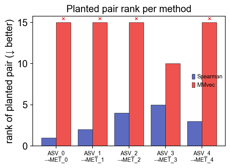
8. Validation — do the methods recover known truth?#
Real data has no ground truth, so to calibrate how much to trust each
method we run them all on ov.micro.simulate_paired, which plants a
configurable set of microbe → metabolite producer pairs with known
effect sizes. Every method should rank the planted pairs above the
~800 random pairs.
ad_mb_sim, ad_mt_sim, truth = ov.micro.simulate_paired(n_pairs=5, seed=0)
res_sp = ov.micro.paired_spearman(ad_mb_sim, ad_mt_sim)
mmvec_sim = ov.micro.MMvec(n_latent=3, epochs=400, val_frac=0.1, seed=0).fit(ad_mb_sim, ad_mt_sim)
ov.micro.plot_paired_method_comparison(truth, spearman_df=res_sp, mmvec_model=mmvec_sim)
plt.tight_layout(); plt.show()
9. Recipe — which method when#
Scenario |
First choice |
|---|---|
Quick screen on a small cohort (< 30 samples) |
Spearman on CLR — fastest, easy FDR, mature |
You want a global “are the two modalities coupled at all?” answer |
CCA — canonical correlations + interpretable loadings |
Compositionally-robust pair-level hypotheses for a paper |
MMvec — unaffected by either table’s normalisation; the paper-reported co-occurrence currency |
Publishable biomarker set |
Intersection of Spearman FDR hits and MMvec top- |
Assumptions each method makes explicit
Spearman-on-CLR assumes the CLR lift accounts for microbial compositionality; it does not help if the metabolite table is also proportion-normalised.
CCA assumes the joint covariance is well-represented by a low-rank linear map. For sample-poor data, prefer
sklearn.cross_decomposition.PLSCanonicalwith a shrinkage prior.MMvec assumes the conditional
P(met | mb)is stationary across samples. If you have strong batch effects, fit per-batch or add a batch covariate to the logits.
For multi-thousand-feature tables the upstream pip install mmvec
package uses negative sampling for scalability; ov.micro.MMvec is
optimised for mid-size studies like this Franzosa example.
References#
Franzosa, E. A., Sirota-Madi, A., Avila-Pacheco, J., Fornelos, N., Haiser, H. J., Reinker, S., Vatanen, T., Hall, A. B., Mallick, H., McIver, L. J., Sauk, J. S., Wilson, R. G., Stevens, B. W., Scott, J. M., Pierce, K., Deik, A. A., Bullock, K., Imhann, F., Porter, J. A., … Xavier, R. J. (2019). Gut microbiome structure and metabolic activity in inflammatory bowel disease. Nature Microbiology, 4(2), 293–305. https://doi.org/10.1038/s41564-018-0306-4
Morton, J. T., Aksenov, A. A., Nothias, L. F., Foulds, J. R., Quinn, R. A., Badri, M. H., Swenson, T. L., Van Goethem, M. W., Northen, T. R., Vazquez-Baeza, Y., Wang, M., Bokulich, N. A., Watters, A., Song, S. J., Bonneau, R., Dorrestein, P. C., & Knight, R. (2019). Learning representations of microbe-metabolite interactions. Nature Methods, 16(12), 1306–1314. https://doi.org/10.1038/s41592-019-0616-3
Muller, E., Shiryan, I., & Borenstein, E. (2024). Multi-omic integration of microbiome data for identifying disease-associated modules. Nature Communications, 15(1), 2621 (curated dataset repo). https://doi.org/10.1038/s41467-024-46869-6
Aitchison, J. (1982). The statistical analysis of compositional data. Journal of the Royal Statistical Society Series B, 44(2), 139–177.