DADA2 backend: pure-Python ASV inference#
The default ov.alignment.amplicon_16s_pipeline backend is UNOISE3
(via vsearch) — fast and benchmark-competitive. This notebook
demonstrates the DADA2 backend, powered by the pure-Python
pydada2 port (no R, no rpy2).
Why a second backend? The canonical R DADA2 (Callahan et al. 2016) is what much of the published 16S literature uses; reviewers sometimes ask for its specific error-model-aware denoising even when UNOISE3 is equivalent on benchmarks. Having both lets users meet that requirement without leaving Python.
Install:
pip install pydada2
One-liner:
adata = ov.alignment.amplicon_16s_pipeline(
    fastq_dir='raw/',
    workdir='/scratch/.../run_dada2',
    backend='dada2',                      # ← switch backend
    db_fasta='/scratch/.../rdp_16s_v18.fa.gz',
)
1. Setup#
from pathlib import Path
import re
import numpy as np
import pandas as pd
import matplotlib.pyplot as plt
import anndata as ad
import omicverse as ov

ov.plot_set()

ROOT = Path('/scratch/users/steorra/analysis/omicverse_dev/cache/16s')
RAW  = ROOT / 'raw' / 'MiSeq_SOP'
DB   = '/scratch/users/steorra/analysis/omicverse_dev/db/rdp/rdp_16s_v18.fa.gz'
WORK = ROOT / 'run_dada2_tutorial'
WORK.mkdir(parents=True, exist_ok=True)
🔬 Starting plot initialization...
🧬 Detecting GPU devices…
✅ NVIDIA CUDA GPUs detected: 1
    • [CUDA 0] NVIDIA H100 80GB HBM3
      Memory: 79.1 GB | Compute: 9.0

   ____            _     _    __
  / __ \____ ___  (_)___| |  / /__  _____________
 / / / / __ `__ \/ / ___/ | / / _ \/ ___/ ___/ _ \
/ /_/ / / / / / / / /__ | |/ /  __/ /  (__  )  __/
\____/_/ /_/ /_/_/\___/ |___/\___/_/  /____/\___/

🔖 Version: 2.1.2rc1   📚 Tutorials: https://omicverse.readthedocs.io/
✅ plot_set complete.
2. Sample selection#
DADA2 is about 2–4× slower than UNOISE3 because of its position-aware error model. For a tutorial we pick the first 6 mothur SOP samples (3 Early + 3 Late + Mock) — enough to show real group structure without a half-hour runtime.
PICK = ['F3D0', 'F3D1', 'F3D2', 'F3D141', 'F3D142', 'F3D143', 'Mock']
samples = []
for name in PICK:
    fq1s = sorted(RAW.glob(f'{name}_S*_L001_R1_001.fastq'))
    if not fq1s:
        continue
    fq1 = fq1s[0]
    fq2 = RAW / fq1.name.replace('_R1_001', '_R2_001')
    samples.append((name, str(fq1), str(fq2)))
print('samples:', [s[0] for s in samples])
samples: ['F3D0', 'F3D1', 'F3D2', 'F3D141', 'F3D142', 'F3D143', 'Mock']
# sample metadata
rows = []
for name, _, _ in samples:
    if name.startswith('F3D'):
        day = int(re.findall(r'F3D(\d+)', name)[0])
        group = 'Early' if day <= 9 else 'Late'
    else:
        day, group = -1, 'Mock'
    rows.append({'sample': name, 'day': day, 'group': group})
meta = pd.DataFrame(rows).set_index('sample')
meta
        day  group
sample
F3D0      0  Early
F3D1      1  Early
F3D2      2  Early
F3D141  141   Late
F3D142  142   Late
F3D143  143   Late
Mock     -1   Mock
3. Run the DADA2 backend#
amplicon_16s_pipeline(backend='dada2') dispatches to
ov.alignment.dada2_pipeline after optional cutadapt trimming
(skipped here — mothur SOP ships pre-trimmed).
Under the hood:
filter_and_trim— quality trim each sample to 240/160 bp, max 2 expected errorslearn_errors— self-consistent error model fit on all F reads, then all R readsdada(per sample) — divisive denoising on dereplicated readsmerge_pairs— merge paired-end reads using the denoiser outputmake_sequence_table— sample × ASV-sequence tableremove_bimera_denovo— consensus chimera removalAssemble AnnData + SINTAX taxonomy on the ASV FASTA
import time
t0 = time.time()
adata_dada2 = ov.alignment.amplicon_16s_pipeline(
    samples=samples,
    workdir=str(WORK),
    db_fasta=DB,
    backend='dada2',
    primer_fwd=None, primer_rev=None,   # mothur SOP is pre-trimmed
    filter_max_ee=2.0,
    sintax_cutoff=0.8,
    threads=4,
    sample_metadata=meta,
)
print(f't = {time.time()-t0:.1f}s  adata = {adata_dada2.shape}  reads = {int(adata_dada2.X.sum())}')
11068560 total bases in 46119 reads from 7 samples will be used for learning the error rates.
selfConsist round 1: re-estimated error rates.
selfConsist round 2: re-estimated error rates.
selfConsist round 3: re-estimated error rates.
selfConsist round 4: re-estimated error rates.
selfConsist converged after 5 round(s).
7379040 total bases in 46119 reads from 7 samples will be used for learning the error rates.
selfConsist round 1: re-estimated error rates.
selfConsist round 2: re-estimated error rates.
selfConsist round 3: re-estimated error rates.
selfConsist converged after 4 round(s).
>> /home/users/steorra/miniforge3/envs/omicverse/bin/vsearch --sintax /scratch/users/steorra/analysis/omicverse_dev/cache/16s/run_dada2_tutorial/asv/asvs.fasta --db /scratch/users/steorra/analysis/omicverse_dev/db/rdp/rdp_16s_v18.fa.gz --tabbedout /scratch/users/steorra/analysis/omicverse_dev/cache/16s/run_dada2_tutorial/taxonomy/sintax.tsv --sintax_cutoff 0.8 --strand both --threads 4
t = 745.0s  adata = (7, 192)  reads = 42533
adata_dada2.var[['phylum','class','genus','sintax_confidence']].head(10)
              phylum        class        genus  sintax_confidence
asv
ASV1   Bacteroidetes  Bacteroidia  Duncaniella               1.00
ASV2   Bacteroidetes  Bacteroidia  Duncaniella               0.99
ASV3   Bacteroidetes  Bacteroidia                            0.79
ASV4   Bacteroidetes  Bacteroidia    Alistipes               1.00
ASV5   Bacteroidetes  Bacteroidia                            0.48
ASV6   Bacteroidetes  Bacteroidia                            0.42
ASV7   Bacteroidetes  Bacteroidia                            0.56
ASV8   Bacteroidetes  Bacteroidia  Bacteroides               1.00
ASV9   Bacteroidetes  Bacteroidia                            0.77
ASV10  Bacteroidetes  Bacteroidia                            0.36
4. Downstream (reuses ov.micro)#
The DADA2 pipeline returns the same AnnData schema as the UNOISE3
backend, so every ov.micro helper works without modification.
# alpha diversity
min_depth = int(np.asarray(adata_dada2.X.sum(axis=1)).min())
ov.micro.Alpha(adata_dada2, rarefy_depth=min_depth).run(['shannon', 'observed_otus'])
# beta + PCoA
ov.micro.Beta(adata_dada2, rarefy_depth=min_depth).run(metric='braycurtis')
ov.micro.Ordinate(adata_dada2, dist_key='braycurtis').pcoa(n=3)
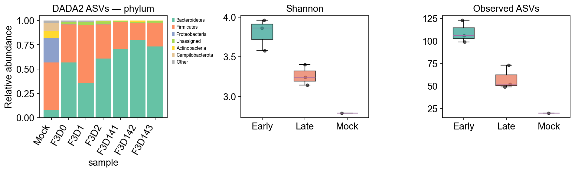
adata_dada2.obs[['day','group','shannon','observed_otus']]
        day  group   shannon  observed_otus
sample
F3D0      0  Early  3.860640            106
F3D1      1  Early  3.961006             99
F3D2      2  Early  3.576407            123
F3D141  141   Late  3.404435             73
F3D142  142   Late  3.143007             49
F3D143  143   Late  3.243364             52
Mock     -1   Mock  2.790998             20
palette = {'Early': '#2a9d8f', 'Late': '#e76f51', 'Mock': '#264653'}
groups = ['Early', 'Late', 'Mock']

fig, axes = plt.subplots(1, 3, figsize=(12, 3.8))
# 1. phylum-level taxonomy stacked bar
from scipy import sparse as _sp
X = adata_dada2.X.toarray() if _sp.issparse(adata_dada2.X) else np.asarray(adata_dada2.X)
phy = adata_dada2.var['phylum'].replace('', 'Unassigned').values
pdf = pd.DataFrame(X, index=adata_dada2.obs_names, columns=phy).T.groupby(level=0).sum().T
pdf = pdf.div(pdf.sum(axis=1), axis=0).fillna(0)
order = adata_dada2.obs.sort_values('day').index
top = pdf.sum().sort_values(ascending=False).head(6).index.tolist()
pplot = pdf[top].loc[order].copy()
pplot['Other'] = 1 - pplot.sum(axis=1)
pplot.plot(kind='bar', stacked=True, ax=axes[0], width=0.9,
           color=plt.cm.Set2(np.linspace(0,1,len(pplot.columns))))
axes[0].set_title('DADA2 ASVs — phylum')
axes[0].set_ylabel('Relative abundance')
axes[0].legend(bbox_to_anchor=(1.02,1), loc='upper left', fontsize=7)
plt.setp(axes[0].get_xticklabels(), rotation=60, ha='right')

# 2. Shannon + Observed boxes
for ax, metric, ylabel in zip(axes[1:], ['shannon', 'observed_otus'],
                              ['Shannon', 'Observed ASVs']):
    data = [adata_dada2.obs[adata_dada2.obs.group==g][metric].dropna().values for g in groups]
    bp = ax.boxplot(data, labels=groups, patch_artist=True, widths=0.5, showfliers=False)
    for patch, g in zip(bp['boxes'], groups):
        patch.set_facecolor(palette[g]); patch.set_alpha(0.7)
    for i, (g, vals) in enumerate(zip(groups, data), start=1):
        x = np.random.normal(i, 0.05, size=len(vals))
        ax.scatter(x, vals, color='k', alpha=0.6, s=18)
    ax.set_title(ylabel)
plt.tight_layout()
plt.show()
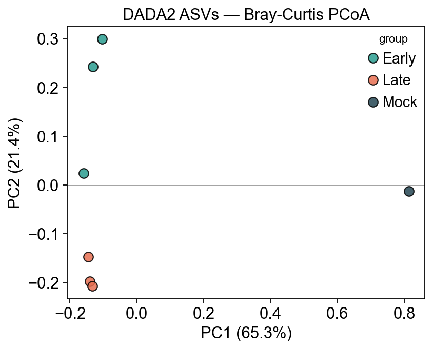
5. PCoA on DADA2 ASVs#
coords = pd.DataFrame(adata_dada2.obsm['braycurtis_pcoa'],
                      index=adata_dada2.obs_names, columns=['PC1','PC2','PC3'])
pct = adata_dada2.uns['micro']['braycurtis_pcoa_var'] * 100

fig, ax = plt.subplots(figsize=(5.5, 4.5))
for g in groups:
    sub = adata_dada2.obs[adata_dada2.obs.group == g]
    if sub.empty: continue
    ax.scatter(coords.loc[sub.index, 'PC1'],
               coords.loc[sub.index, 'PC2'],
               color=palette[g], s=70, alpha=0.85, edgecolor='k', label=g)
ax.set_xlabel(f'PC1 ({pct[0]:.1f}%)')
ax.set_ylabel(f'PC2 ({pct[1]:.1f}%)')
ax.set_title('DADA2 ASVs — Bray-Curtis PCoA')
ax.legend(title='group')
ax.axhline(0, color='k', lw=0.4, alpha=0.4)
ax.axvline(0, color='k', lw=0.4, alpha=0.4)
plt.tight_layout()
plt.show()
Notes#
When to pick DADA2 over UNOISE3? If a journal / reviewer explicitly requires DADA2-style error-model denoising for reproducibility with the original paper’s pipeline. On benchmarks (Vestergaard 2024 ISME Comms) UNOISE3 ≈ DADA2 for biological signal recovery, with UNOISE3 ~3× faster.
Performance.
pydada2.dadais ~1–2× slower than the R/C++ DADA2 (pure Python, no Cython yet). Acceptable for <200 samples.Taxonomy. This tutorial reuses the SINTAX reference we already built for the UNOISE3 tutorial — the DADA2 ASV FASTA is piped through
ov.alignment.vsearch.sintax. For DADA2-native RDP naive Bayes, usepydada2.assign_taxonomywith a DADA2-formatted training set (e.g.silva_nr99_v138.1_wSpecies_train_set.fa.gz).