GeneModule Identified#
In omicverse, we prepared two methods to identify the gene module, one is cNMF, the other one is hospot.
import scanpy as sc
import omicverse as ov
ov.style(font_path='Arial')

%load_ext autoreload
%autoreload 2
🔬 Starting plot initialization...
Using already downloaded Arial font from: /tmp/omicverse_arial.ttf
Registered as: Arial
🧬 Detecting GPU devices…
✅ NVIDIA CUDA GPUs detected: 1
    • [CUDA 0] NVIDIA H100 80GB HBM3
      Memory: 79.1 GB | Compute: 9.0

   ____            _     _    __
  / __ \____ ___  (_)___| |  / /__  _____________
 / / / / __ `__ \/ / ___/ | / / _ \/ ___/ ___/ _ \
/ /_/ / / / / / / / /__ | |/ /  __/ /  (__  )  __/
\____/_/ /_/ /_/_/\___/ |___/\___/_/  /____/\___/

🔖 Version: 1.7.9rc1   📚 Tutorials: https://omicverse.readthedocs.io/
✅ plot_set complete.
Loading dataset#
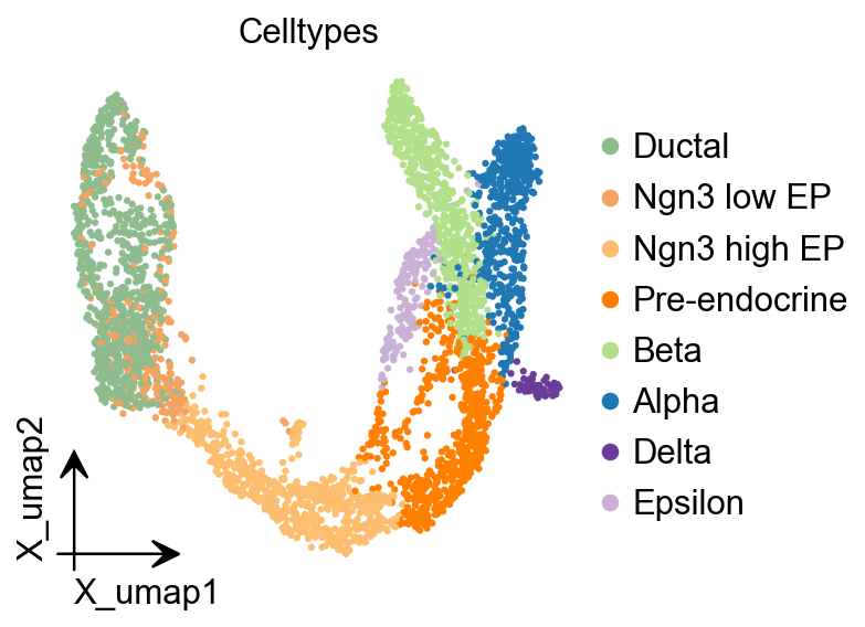
Here, we use the dentategyrus dataset as an example for cNMF or Hospot.
adata=ov.datasets.pancreatic_endocrinogenesis()
🔍 Downloading data to ./data/endocrinogenesis_day15.h5ad
⚠️ File ./data/endocrinogenesis_day15.h5ad already exists
 Loading data from ./data/endocrinogenesis_day15.h5ad
✅ Successfully loaded: 3696 cells × 27998 genes
%%time
adata=ov.pp.preprocess(adata,mode='shiftlog|pearson',n_HVGs=2000,)
adata
🔍 [2026-01-07 17:06:35] Running preprocessing in 'cpu' mode...
Begin robust gene identification
    After filtration, 17750/27998 genes are kept.
    Among 17750 genes, 16426 genes are robust.
✅ Robust gene identification completed successfully.
Begin size normalization: shiftlog and HVGs selection pearson

🔍 Count Normalization:
   Target sum: 500000.0
   Exclude highly expressed: True
   Max fraction threshold: 0.2
   ⚠️ Excluding 1 highly-expressed genes from normalization computation
   Excluded genes: ['Ghrl']

✅ Count Normalization Completed Successfully!
   ✓ Processed: 3,696 cells × 16,426 genes
   ✓ Runtime: 0.25s

🔍 Highly Variable Genes Selection (Experimental):
   Method: pearson_residuals
   Target genes: 2,000
   Theta (overdispersion): 100

✅ Experimental HVG Selection Completed Successfully!
   ✓ Selected: 2,000 highly variable genes out of 16,426 total (12.2%)
   ✓ Results added to AnnData object:
     • 'highly_variable': Boolean vector (adata.var)
     • 'highly_variable_rank': Float vector (adata.var)
     • 'highly_variable_nbatches': Int vector (adata.var)
     • 'highly_variable_intersection': Boolean vector (adata.var)
     • 'means': Float vector (adata.var)
     • 'variances': Float vector (adata.var)
     • 'residual_variances': Float vector (adata.var)
    Time to analyze data in cpu: 1.11 seconds.
✅ Preprocessing completed successfully.
    Added:
        'highly_variable_features', boolean vector (adata.var)
        'means', float vector (adata.var)
        'variances', float vector (adata.var)
        'residual_variances', float vector (adata.var)
        'counts', raw counts layer (adata.layers)
    End of size normalization: shiftlog and HVGs selection pearson
CPU times: user 1.43 s, sys: 717 ms, total: 2.15 s
Wall time: 1.51 s
AnnData object with n_obs × n_vars = 3696 × 16426
    obs: 'clusters_coarse', 'clusters', 'S_score', 'G2M_score'
    var: 'highly_variable_genes', 'n_cells', 'percent_cells', 'robust', 'highly_variable_features', 'means', 'variances', 'residual_variances', 'highly_variable_rank', 'highly_variable'
    uns: 'clusters_coarse_colors', 'clusters_colors', 'day_colors', 'neighbors', 'pca', 'log1p', 'hvg', 'status', 'status_args', 'REFERENCE_MANU'
    obsm: 'X_pca', 'X_umap'
    layers: 'spliced', 'unspliced', 'counts'
    obsp: 'distances', 'connectivities'
ov.pp.scale(adata)
ov.pp.pca(adata)
computing PCA🔍
    with n_comps=50
   🖥️ Using sklearn PCA for CPU computation
   🖥️ sklearn PCA backend: CPU computation
    finished✅ (0:00:02)
import matplotlib.pyplot as plt
from matplotlib import patheffects
fig, ax = plt.subplots(figsize=(4,4))
ov.pl.embedding(
    adata,
    basis="X_umap",
    color=['clusters'],
    frameon='small',
    title="Celltypes",
    #legend_loc='on data',
    legend_fontsize=14,
    legend_fontoutline=2,
    #size=10,
    ax=ax,
    #legend_loc=True,
    add_outline=False,
    #add_outline=True,
    outline_color='black',
    outline_width=1,
    show=False,
)
<Axes: title={'center': 'Celltypes'}, xlabel='X_umap1', ylabel='X_umap2'>
Consensus Non-negative Matrix factorization (cNMF)#
cNMF is an analysis pipeline for inferring gene expression programs from single-cell RNA-Seq (scRNA-Seq) data.
It takes a count matrix (N cells X G genes) as input and produces a (K x G) matrix of gene expression programs (GEPs) and a (N x K) matrix specifying the usage of each program for each cell in the data. You can read more about the method in the github and check out examples on dentategyrus.
Dylan KotliarAdrian VeresM Aurel NagyShervin TabriziEran HodisDouglas A MeltonPardis C Sabeti (2019) Identifying gene expression programs of cell-type identity and cellular activity with single-cell RNA-Seq eLife 8:e43803.
Initialize and Training model#
In omicverse, you can set use_gpu=True to perform the NMF analysis using torchnmf package, it’s easy to install using pip install torchnmf. But it should be noticed the accurancy is different if you use use_gpu=True mode.
import numpy as np
## Initialize the cnmf object that will be used to run analyses
cnmf_obj = ov.single.cNMF(
    adata,components=np.arange(5,15), n_iter=20,
    seed=14, num_highvar_genes=2000,
    output_dir=None, name='pancrea_cNMF',use_gpu=True
)
normalizing counts per cell
    finished (0:00:00)
## Specify that the jobs are being distributed over a single worker (total_workers=1) and then launch that worker
cnmf_obj.factorize(worker_i=0, total_workers=1)
🚀 Running NMF on GPU (device 0)
Running 200 factorization iterations for worker 0...
✓ Worker 0 completed 200 iterations. Total in memory: 200
if u want to accerlate the calculation, you can try the code below
#cnmf_obj.factorize(worker_i=0, total_workers=2)
#cnmf_obj.factorize(worker_i=1, total_workers=2)
cnmf_obj.combine(skip_missing_files=True)
Combining factorizations for k=5.
  Found all 20 iterations for k=5
Combining factorizations for k=6.
  Found all 20 iterations for k=6
Combining factorizations for k=7.
  Found all 20 iterations for k=7
Combining factorizations for k=8.
  Found all 20 iterations for k=8
Combining factorizations for k=9.
  Found all 20 iterations for k=9
Combining factorizations for k=10.
  Found all 20 iterations for k=10
Combining factorizations for k=11.
  Found all 20 iterations for k=11
Combining factorizations for k=12.
  Found all 20 iterations for k=12
Combining factorizations for k=13.
  Found all 20 iterations for k=13
Combining factorizations for k=14.
  Found all 20 iterations for k=14
cnmf_obj.save('test/cnmf_obj.pkl')
✓ cNMF object saved to: test/cnmf_obj.pkl
  - 200 factorization iterations
  - 10 merged spectra (K values)
  - 0 consensus results
cnmf_obj.load('test/cnmf_obj.pkl')
📂 Load Operation:
   Source path: test/cnmf_obj.pkl
   Using: pickle
   ✅ Successfully loaded!
   Loaded object type: cNMF
────────────────────────────────────────────────────────────
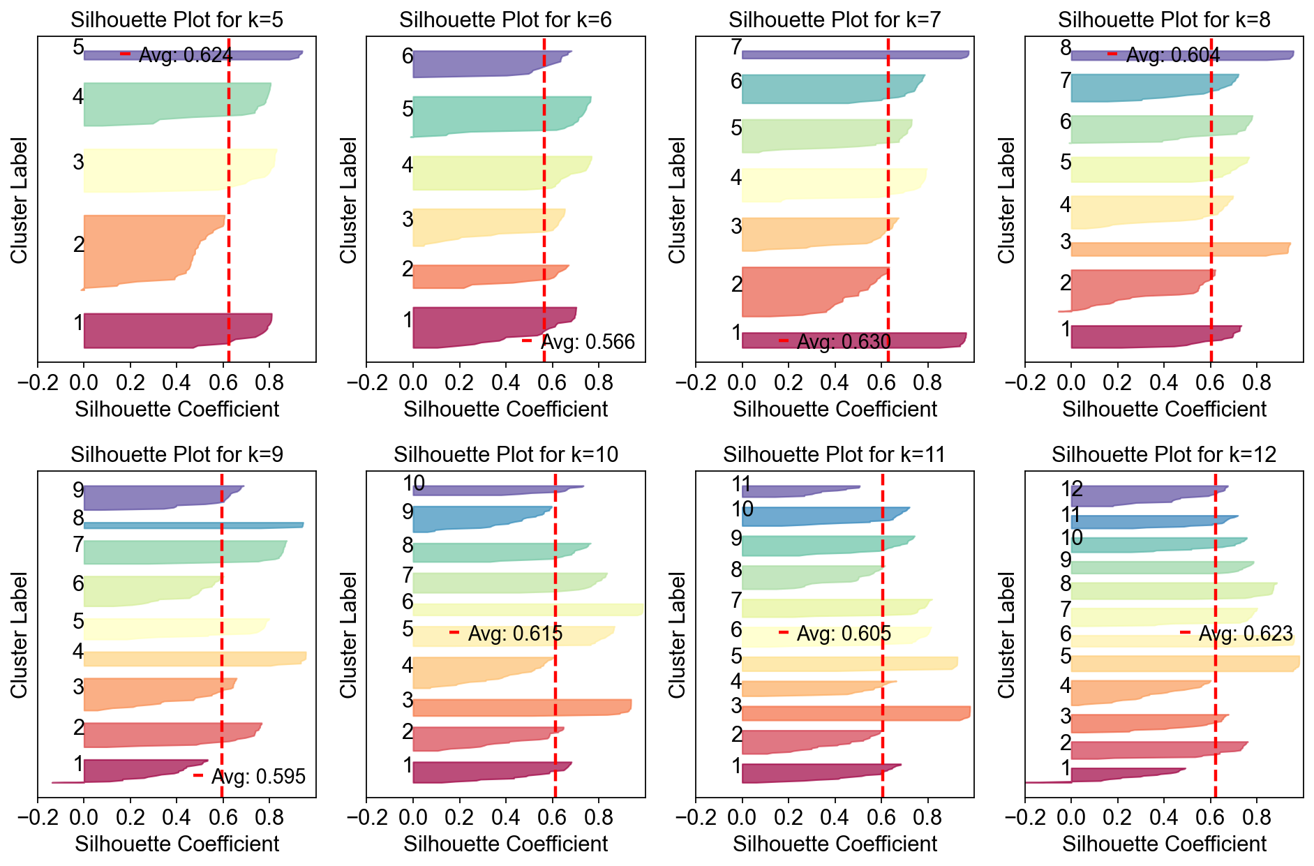
Compute the stability and error at each choice of K to see if a clear choice jumps out.#
Please note that the maximum stability solution is not always the best choice depending on the application. However it is often a good starting point even if you have to investigate several choices of K
sil_data = cnmf_obj.calculate_silhouette_k(k=7, density_threshold=2.0)

print(f"Average silhouette score: {sil_data['avg_silhouette']:.4f}")
print(f"Per-sample scores: {sil_data['silhouette_values']}")
print(f"Cluster labels: {sil_data['cluster_labels']}")
Average silhouette score: 0.6299
Per-sample scores: [0.7106916  0.5630814  0.9380699  0.9647325  0.7674971  0.6231896
 0.7462224  0.37565622 0.6270655  0.06985006 0.57842237 0.7953116
 0.6916376  0.78109527 0.7101993  0.55603576 0.7441653  0.75451505
 0.5479283  0.9625558  0.39097318 0.43278462 0.97507685 0.60460097
 0.7781605  0.67471343 0.53983855 0.76693016 0.64284235 0.41358513
 0.7894957  0.5756324  0.9714798  0.54308915 0.73912    0.5916759
 0.29305577 0.5943038  0.9639678  0.75087273 0.4957365  0.7721111
 0.5499817  0.5790103  0.73023146 0.588068   0.77418405 0.18887511
 0.3828089  0.71155    0.93825644 0.66316015 0.7878561  0.9744356
 0.7274356  0.628735   0.96383363 0.63263124 0.64927    0.17515936
 0.7908563  0.59846324 0.67699015 0.37909067 0.7533861  0.27464965
 0.94846934 0.56372494 0.62612045 0.39772192 0.4309683  0.50130105
 0.5352081  0.2945753  0.7588943  0.7905221  0.7286009  0.94101614
 0.5963504  0.60703915 0.6570392  0.17053658 0.7238535  0.63654566
 0.164855   0.60783756 0.70025706 0.64824665 0.08693045 0.70052814
 0.6865447  0.5977072  0.95368004 0.7289692  0.44170102 0.7777483
 0.7743478  0.4995771  0.69891447 0.580345   0.78578705 0.3635015
 0.71654373 0.9585754  0.6125389  0.629792   0.6913672  0.4552708
 0.10541853 0.96240723 0.38784292 0.6745267  0.79051185 0.70214224
 0.84903276 0.6250461  0.509497   0.055472   0.6147614  0.49948195
 0.25953737 0.72868174 0.7900021  0.6660114  0.360943   0.6711156
 0.7861118  0.9580041  0.57364947 0.43281323 0.78196883 0.64617914
 0.50612485 0.1185286  0.7382589  0.9742657  0.67354196 0.76530886
 0.5728536  0.7114021 ]
Cluster labels: [4 2 0 6 3 1 5 1 2 4 1 3 4 5 4 2 5 3 1 0 1 1 6 2 5 4 1 3 2 1 3 4 6 1 5 1 1
 2 0 5 4 3 1 2 4 3 5 3 1 5 0 2 3 6 4 1 0 1 2 4 3 5 4 4 5 2 0 1 3 1 1 1 2 2
 5 3 4 6 1 5 2 3 4 3 3 1 5 2 4 3 4 2 0 4 1 3 5 1 5 1 3 1 4 0 2 1 3 5 2 0 2
 4 3 4 0 1 5 2 2 1 1 4 3 2 1 5 5 0 4 1 3 2 1 1 3 6 2 5 1 4]
fig, axes = plt.subplots(2,4,figsize=(12,8))
for k,ax in zip(np.arange(5,15),axes.flatten()):
    cnmf_obj.plot_silhouette_for_k(
        k=k,
        density_threshold=2.0,
        show_avg=True,
        cmap='Spectral',ax=ax
    )
plt.tight_layout()
fig=cnmf_obj.k_selection_plot(close_fig=False)
Calculating silhouette scores for K selection...
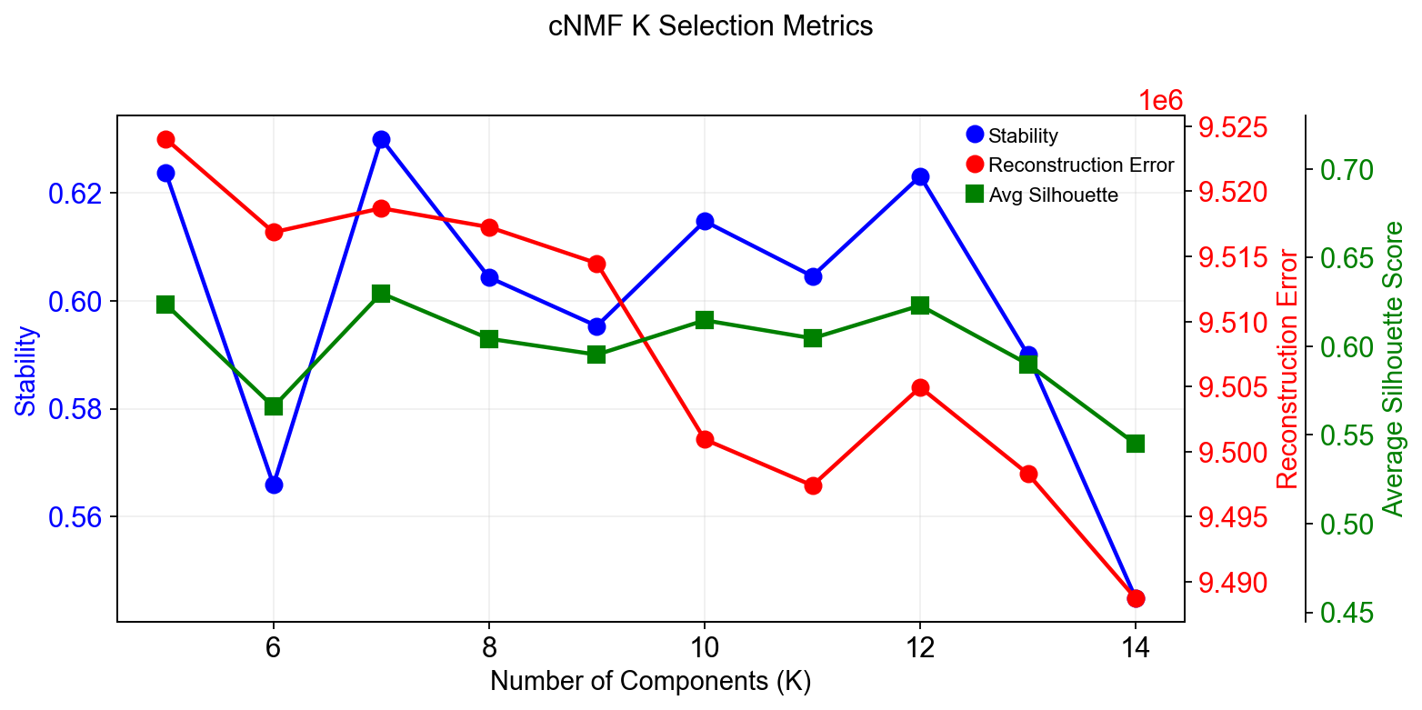
In this range, K=12 gave the most stable solution so we will begin by looking at that.
The next step computes the consensus solution for a given choice of K. We first run it without any outlier filtering to see what that looks like. Setting the density threshold to anything >= 2.00 (the maximum possible distance between two unit vectors) ensures that nothing will be filtered.
Then we run the consensus with a filter for outliers determined based on inspecting the histogram of distances between components and their nearest neighbors
selected_K = 12
density_threshold = 2.00
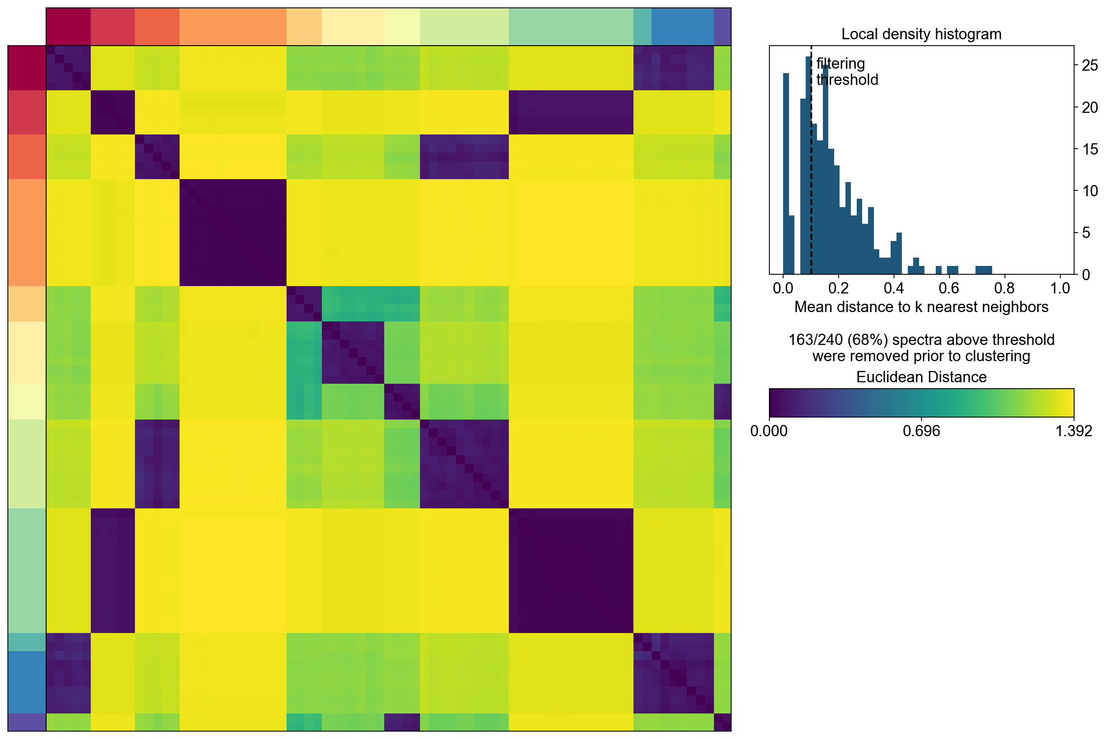
cnmf_obj.consensus(k=selected_K,
                   density_threshold=density_threshold,
                   show_clustering=True,
                   close_clustergram_fig=False)
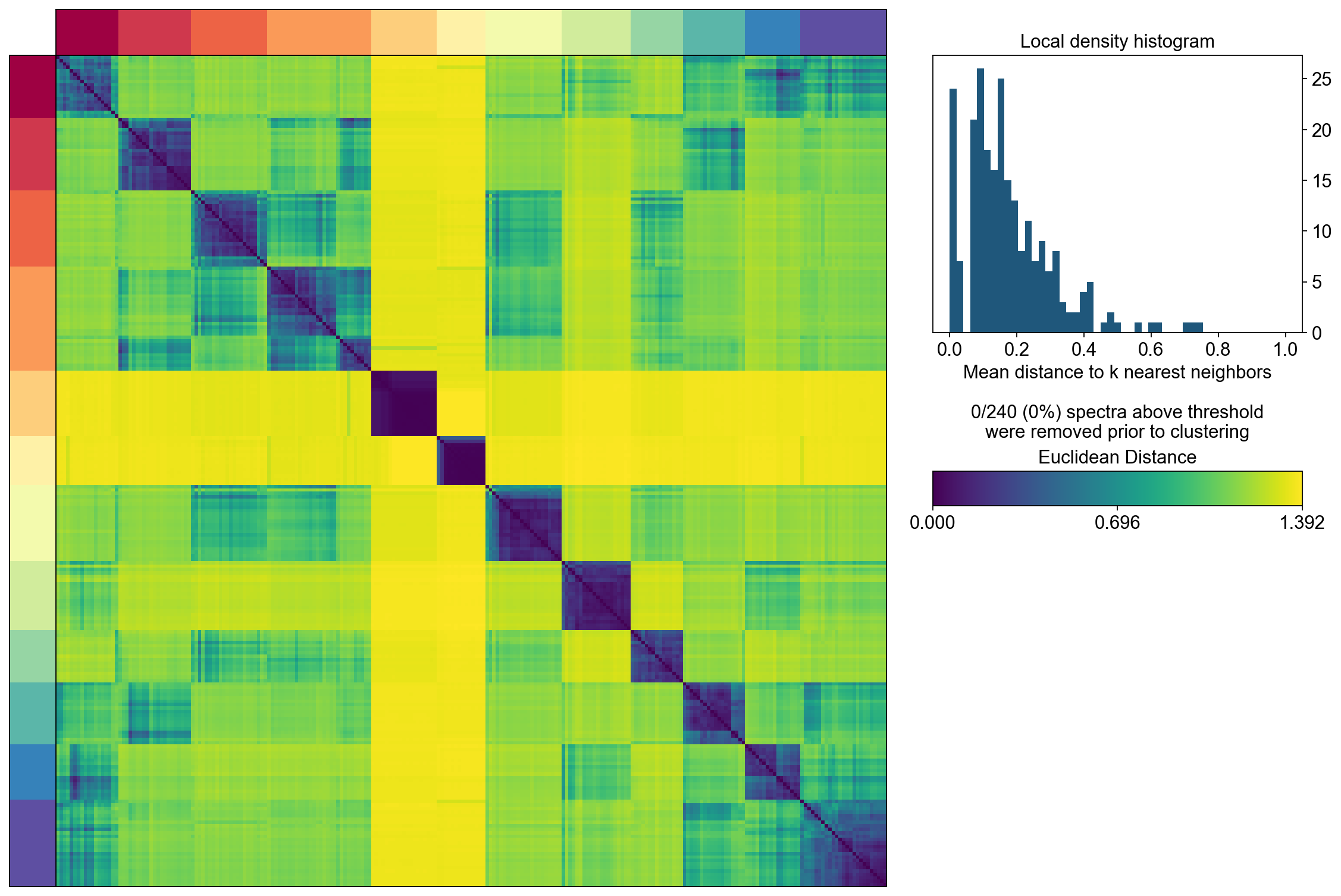
The above consensus plot shows that there is a substantial degree of concordance between the replicates with a few outliers. An outlier threshold of 0.1 seems appropriate
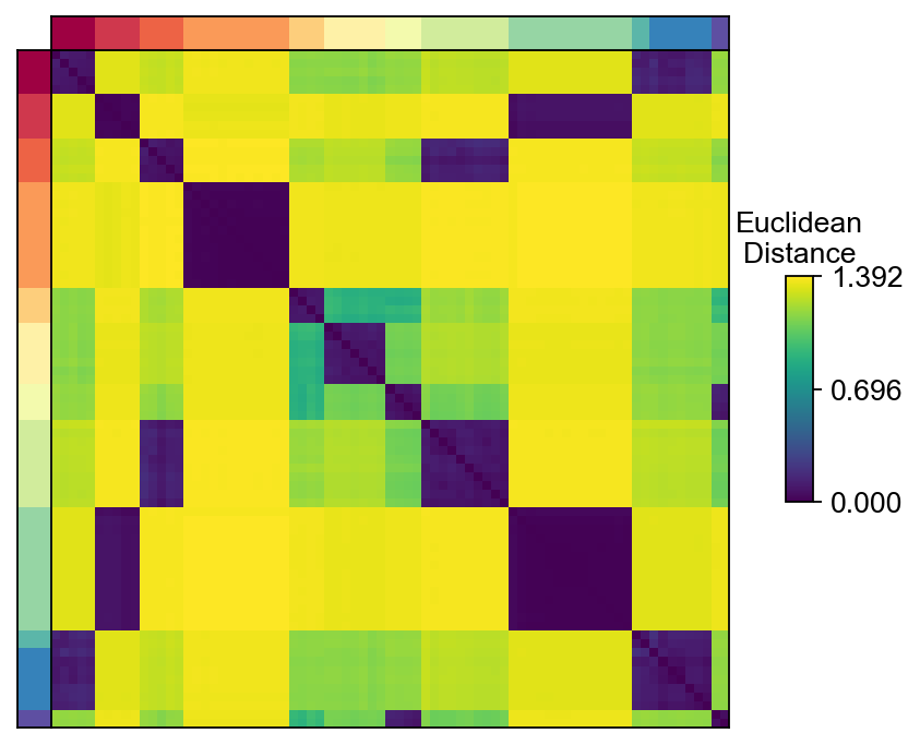
density_threshold = 0.10
cnmf_obj.consensus(k=selected_K,
                   density_threshold=density_threshold,
                   show_clustering=True,
                   close_clustergram_fig=False)
Visualization the result#
import seaborn as sns
import matplotlib.pyplot as plt
from matplotlib import patheffects

from matplotlib import gridspec
import matplotlib.pyplot as plt

width_ratios = [0.2, 4, 0.5, 10, 1]
height_ratios = [0.2, 4]
fig = plt.figure(figsize=(sum(width_ratios), sum(height_ratios)))
gs = gridspec.GridSpec(len(height_ratios), len(width_ratios), fig,
                        0.01, 0.01, 0.98, 0.98,
                       height_ratios=height_ratios,
                       width_ratios=width_ratios,
                       wspace=0, hspace=0)

D = cnmf_obj.topic_dist[cnmf_obj.spectra_order, :][:, cnmf_obj.spectra_order]
dist_ax = fig.add_subplot(gs[1,1], xscale='linear', yscale='linear',
                                      xticks=[], yticks=[],xlabel='', ylabel='',
                                      frameon=True)
dist_im = dist_ax.imshow(D, interpolation='none', cmap='viridis',
                         aspect='auto', rasterized=True)

left_ax = fig.add_subplot(gs[1,0], xscale='linear', yscale='linear', xticks=[], yticks=[],
                xlabel='', ylabel='', frameon=True)
left_ax.imshow(cnmf_obj.kmeans_cluster_labels.values[cnmf_obj.spectra_order].reshape(-1, 1),
                            interpolation='none', cmap='Spectral', aspect='auto',
                            rasterized=True)

top_ax = fig.add_subplot(gs[0,1], xscale='linear', yscale='linear', xticks=[], yticks=[],
                xlabel='', ylabel='', frameon=True)
top_ax.imshow(cnmf_obj.kmeans_cluster_labels.values[cnmf_obj.spectra_order].reshape(1, -1),
                  interpolation='none', cmap='Spectral', aspect='auto',
                    rasterized=True)

cbar_gs = gridspec.GridSpecFromSubplotSpec(3, 3, subplot_spec=gs[1, 2],
                                   wspace=0, hspace=0)
cbar_ax = fig.add_subplot(cbar_gs[1,2], xscale='linear', yscale='linear',
    xlabel='', ylabel='', frameon=True, title='Euclidean\nDistance')
cbar_ax.set_title('Euclidean\nDistance',fontsize=12)
vmin = D.min().min()
vmax = D.max().max()
fig.colorbar(dist_im, cax=cbar_ax,
        ticks=np.linspace(vmin, vmax, 3),
        )
cbar_ax.set_yticklabels(cbar_ax.get_yticklabels(),fontsize=12)
[Text(1, 0.0, '0.000'),
 Text(1, 0.6961943507194519, '0.696'),
 Text(1, 1.3923887014389038, '1.392')]
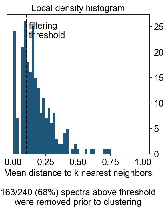
density_filter = cnmf_obj.local_density.iloc[:, 0] < density_threshold
fig, hist_ax = plt.subplots(figsize=(4,4))

#hist_ax = fig.add_subplot(hist_gs[0,0], xscale='linear', yscale='linear',
 #   xlabel='', ylabel='', frameon=True, title='Local density histogram')
hist_ax.hist(cnmf_obj.local_density.values, bins=np.linspace(0, 1, 50))
hist_ax.yaxis.tick_right()

xlim = hist_ax.get_xlim()
ylim = hist_ax.get_ylim()
if density_threshold < xlim[1]:
    hist_ax.axvline(density_threshold, linestyle='--', color='k')
    hist_ax.text(density_threshold  + 0.02, ylim[1] * 0.95, 'filtering\nthreshold\n\n', va='top')
hist_ax.set_xlim(xlim)
hist_ax.set_xlabel('Mean distance to k nearest neighbors\n\n%d/%d (%.0f%%) spectra above threshold\nwere removed prior to clustering'%(sum(~density_filter), len(density_filter), 100*(~density_filter).mean()))
hist_ax.set_title('Local density histogram')
Text(0.5, 1.0, 'Local density histogram')
Explode the cNMF result#
We can load the results for a cNMF run with a given K and density filtering threshold like below
result_dict = cnmf_obj.load_results(K=selected_K, density_threshold=density_threshold)
result_dict['usage_norm'].head()
| cNMF_1 | cNMF_2 | cNMF_3 | cNMF_4 | cNMF_5 | cNMF_6 | cNMF_7 | cNMF_8 | cNMF_9 | cNMF_10 | cNMF_11 | cNMF_12 | |
|---|---|---|---|---|---|---|---|---|---|---|---|---|
| index | ||||||||||||
| AAACCTGAGAGGGATA | 0.052900 | 0.557367 | 0.000422 | 0.021016 | 0.006930 | 0.003447 | 0.079662 | 0.082491 | 0.000638 | 0.005284 | 0.030603 | 0.159242 |
| AAACCTGAGCCTTGAT | 0.020833 | 0.000962 | 0.570114 | 0.043898 | 0.000887 | 0.173351 | 0.007137 | 0.132107 | 0.004638 | 0.000670 | 0.029395 | 0.016007 |
| AAACCTGAGGCAATTA | 0.000142 | 0.306285 | 0.050380 | 0.000632 | 0.017096 | 0.028461 | 0.017249 | 0.053764 | 0.000810 | 0.005584 | 0.131687 | 0.387909 |
| AAACCTGCATCATCCC | 0.011620 | 0.000740 | 0.142481 | 0.011996 | 0.002794 | 0.510735 | 0.001547 | 0.281503 | 0.003506 | 0.025785 | 0.005863 | 0.001429 |
| AAACCTGGTAAGTGGC | 0.543322 | 0.149150 | 0.003397 | 0.199798 | 0.000105 | 0.011512 | 0.023303 | 0.000721 | 0.003200 | 0.022096 | 0.025705 | 0.017692 |
result_dict['gep_scores'].head()
| 1 | 2 | 3 | 4 | 5 | 6 | 7 | 8 | 9 | 10 | 11 | 12 | |
|---|---|---|---|---|---|---|---|---|---|---|---|---|
| index | ||||||||||||
| Xkr4 | -0.007757 | -0.001951 | 0.010988 | 0.000303 | 0.000153 | -0.006076 | 0.001394 | -0.000277 | 0.007163 | -0.000909 | -0.001658 | -0.001580 |
| Mrpl15 | -0.004883 | 0.017592 | -0.018511 | -0.027615 | -0.021772 | 0.037728 | 0.013916 | 0.011741 | -0.016687 | 0.021974 | -0.005451 | -0.004443 |
| Npbwr1 | 0.008097 | 0.001318 | -0.010134 | -0.018095 | -0.016732 | 0.000294 | -0.003005 | 0.000016 | 0.055294 | -0.001144 | -0.000746 | -0.001143 |
| 4732440D04Rik | 0.008619 | -0.005695 | -0.006195 | -0.013188 | 0.014607 | 0.001333 | -0.008327 | -0.001492 | 0.005998 | 0.000943 | 0.000016 | -0.002278 |
| Gm26901 | -0.007764 | 0.026168 | -0.008942 | 0.023266 | -0.009654 | -0.017616 | -0.010079 | 0.009438 | -0.008486 | -0.003649 | -0.001237 | -0.000615 |
result_dict['gep_tpm'].head()
| 1 | 2 | 3 | 4 | 5 | 6 | 7 | 8 | 9 | 10 | 11 | 12 | |
|---|---|---|---|---|---|---|---|---|---|---|---|---|
| index | ||||||||||||
| Xkr4 | 0.000000 | 8.302266e-03 | 1.477936e-02 | 0.000000 | 1.833748e-03 | 3.670955e-05 | 8.236001e-29 | 1.203458e-02 | 0.008952 | 0.000000 | 0.000000e+00 | 0.002387 |
| Mrpl15 | 0.010844 | 4.420368e-19 | 9.274849e-01 | 0.018528 | 5.522656e-01 | 7.091711e-02 | 1.485689e-01 | 3.118949e-02 | 0.046750 | 0.155717 | 5.128206e-14 | 0.662705 |
| Npbwr1 | 0.016931 | 0.000000e+00 | 2.428719e-16 | 0.000000 | 9.940618e-04 | 4.695393e-07 | 0.000000e+00 | 0.000000e+00 | 0.000000 | 0.009431 | 0.000000e+00 | 0.000000 |
| 4732440D04Rik | 0.008692 | 1.156003e-05 | 7.946806e-03 | 0.000000 | 4.226314e-02 | 3.767684e-02 | 3.580834e-02 | 2.182026e-12 | 0.000063 | 0.005495 | 3.885308e-30 | 0.006224 |
| Gm26901 | 0.000000 | 3.010304e-02 | 3.764709e-20 | 0.000000 | 1.401298e-45 | 1.688556e-03 | 8.005813e-03 | 0.000000e+00 | 0.000000 | 0.000000 | 0.000000e+00 | 0.062770 |
result_dict['top_genes'].head()
| 1 | 2 | 3 | 4 | 5 | 6 | 7 | 8 | 9 | 10 | 11 | 12 | |
|---|---|---|---|---|---|---|---|---|---|---|---|---|
| 0 | Hmgn3 | Anxa2 | Nnat | Grin3a | Krt7 | Sox4 | Gmnn | Olfm1 | Ghrl | Birc5 | Prph | Gpr132 |
| 1 | Chgb | Cldn3 | Ppp1r1a | Atoh8 | 1110012L19Rik | Nptx2 | Mcm5 | Selm | Maged2 | Nusap1 | Stmn2 | AB124611 |
| 2 | Rap1b | Krt18 | Ins2 | Enpp2 | BC023829 | Mpzl1 | Pcna | Ppp1r14a | Gm11837 | Cenpf | Hand2 | Tyrobp |
| 3 | Cldn4 | Atp1b1 | Sdf2l1 | Ttr | Gspt1 | Bcl2 | 2810417H13Rik | Tmsb4x | Arg1 | Plk1 | Stmn4 | Fcgr3 |
| 4 | Pax6 | Lurap1l | Iapp | Tmem171 | Cck | Gadd45a | Rrm2 | Shf | Irs4 | Cks2 | Pirt | AI662270 |
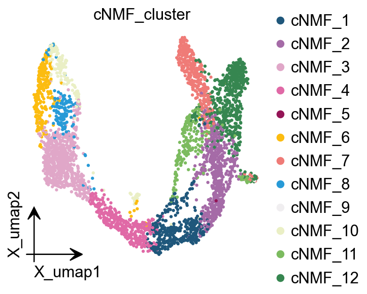
We can extract cell classes directly based on the highest cNMF in each cell, but this has the disadvantage that it will lead to mixed cell classes if the heterogeneity of our data is not as strong as it should be.
cnmf_obj.get_results(adata,result_dict)
cNMF_cluster is added to adata.obs
gene scores are added to adata.var
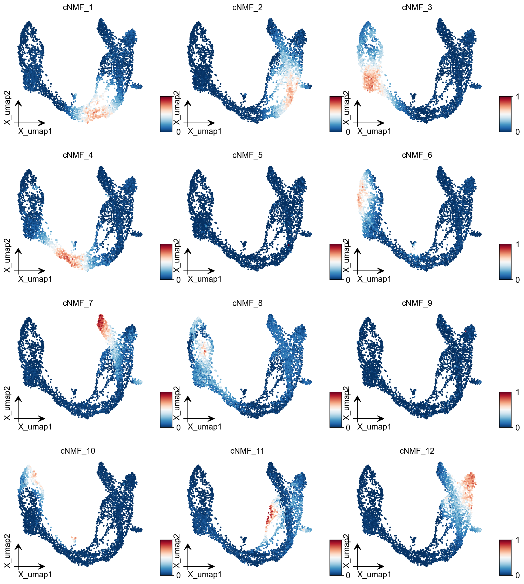
ov.pl.embedding(adata, basis='X_umap',color=result_dict['usage_norm'].columns,
           use_raw=False, ncols=3, vmin=0, vmax=1,frameon='small')
ov.pl.embedding(
    adata,
    basis="X_umap",
    color=['cNMF_cluster'],
    frameon='small',
    #title="Celltypes",
    #legend_loc='on data',
    legend_fontsize=14,
    legend_fontoutline=2,
    #size=10,
    #legend_loc=True,
    add_outline=False,
    #add_outline=True,
    outline_color='black',
    outline_width=1,
    show=False,
)
<Axes: title={'center': 'cNMF_cluster'}, xlabel='X_umap1', ylabel='X_umap2'>
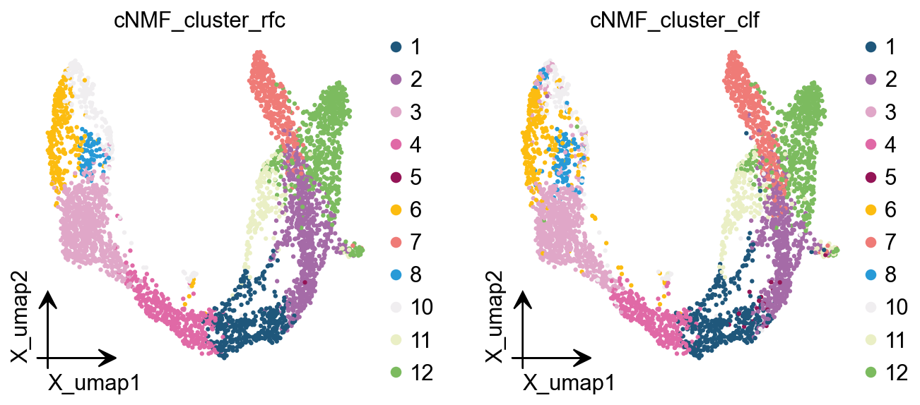
Here we are, proposing another idea of categorisation. We use cells with cNMF greater than 0.5 as a primitive class, and then train a random forest classification model, and then use the random forest classification model to classify cells with cNMF less than 0.5 to get a more accurate
cnmf_obj.get_results_rfc(adata,result_dict,
                         use_rep='scaled|original|X_pca',
                        cNMF_threshold=0.5)
Single Tree: 0.9555555555555556
Random Forest: 0.9873015873015873
cNMF_cluster_rfc is added to adata.obs
cNMF_cluster_clf is added to adata.obs
ov.pl.embedding(
    adata,
    basis="X_umap",
    color=['cNMF_cluster_rfc','cNMF_cluster_clf'],
    frameon='small',
    #title="Celltypes",
    #legend_loc='on data',
    legend_fontsize=14,
    legend_fontoutline=2,
    #size=10,
    #legend_loc=True,
    add_outline=False,
    #add_outline=True,
    outline_color='black',
    outline_width=1,
    show=False,
)
[<Axes: title={'center': 'cNMF_cluster_rfc'}, xlabel='X_umap1', ylabel='X_umap2'>,
 <Axes: title={'center': 'cNMF_cluster_clf'}, xlabel='X_umap1', ylabel='X_umap2'>]
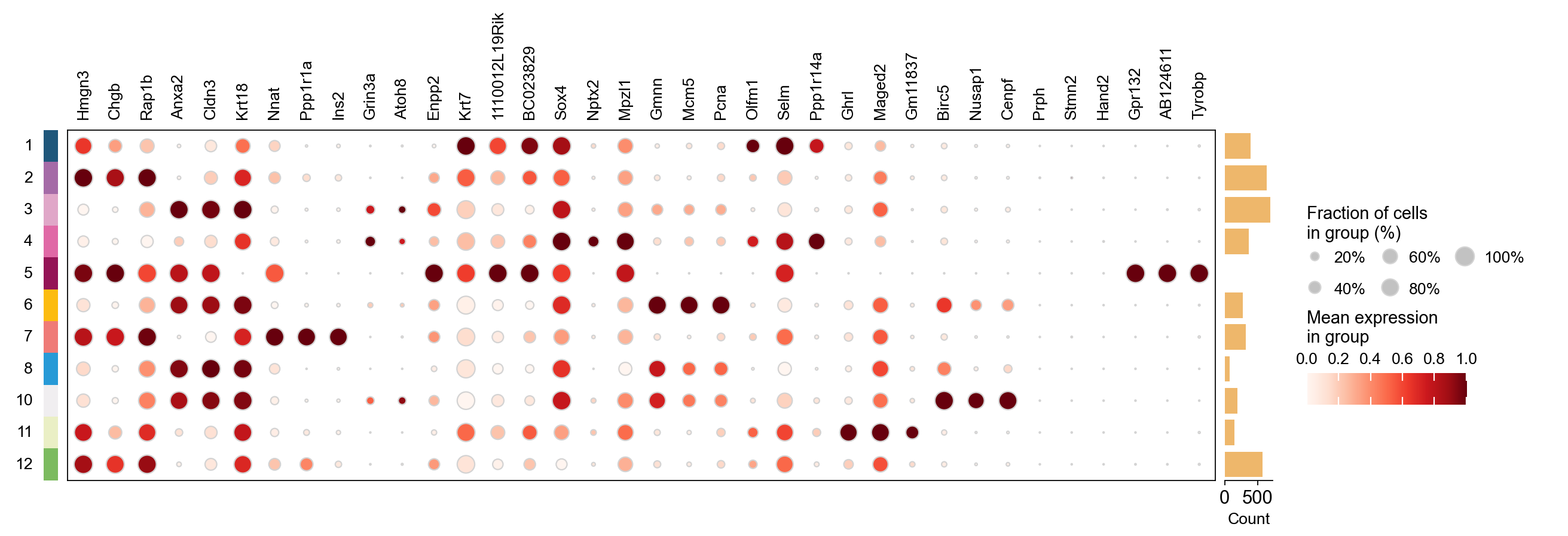
plot_genes=[]
for i in result_dict['top_genes'].columns:
    plot_genes+=result_dict['top_genes'][i][:3].values.reshape(-1).tolist()
ov.pl.dotplot(
    adata,plot_genes,
    "cNMF_cluster_rfc", dendrogram=False,standard_scale='var',
)
<marsilea.heatmap.SizedHeatmap at 0x7f84d0263e20>
Hotspot#
Hotspot is a tool for identifying informative genes (and gene modules) in a single-cell dataset.
DeTomaso D, Yosef N. Hotspot identifies informative gene modules across modalities of single-cell genomics. Cell Syst. 2021 May 19;12(5):446-456.e9. doi: 10.1016/j.cels.2021.04.005. Epub 2021 May 4. PMID: 33951459.
# to calculate the total_counts
sc.pp.calculate_qc_metrics(adata, percent_top=None, log1p=False, inplace=True)
# Create the Hotspot object and the neighborhood graph
# hotspot works a lot faster with a csc matrix!
adata.layers["counts_csc"] = adata.layers["counts"].tocsc()
hs = ov.single.Hotspot(
    adata,
    layer_key="counts_csc",
    model='danb',
    latent_obsm_key="X_pca",
    umi_counts_obs_key="total_counts"
)

hs.create_knn_graph(
    weighted_graph=False, n_neighbors=30,
)
Determining informative genes#
Now we compute autocorrelations for each gene, in the pca-space, to determine which genes have the most informative variation.
hs_results = hs.compute_autocorrelations(jobs=8)

hs_results.head(15)
| C | Z | Pval | FDR | |
|---|---|---|---|---|
| Gene | ||||
| Btbd17 | 0.735443 | 221.872382 | 0.0 | 0.0 |
| Gadd45a | 0.666501 | 213.692549 | 0.0 | 0.0 |
| Neurog3 | 0.658402 | 208.855264 | 0.0 | 0.0 |
| Spp1 | 0.806283 | 200.751152 | 0.0 | 0.0 |
| Mdk | 0.695210 | 199.681646 | 0.0 | 0.0 |
| Rps19 | 0.819013 | 199.041836 | 0.0 | 0.0 |
| Gnas | 0.701187 | 192.850484 | 0.0 | 0.0 |
| Rpl13 | 0.817551 | 192.250551 | 0.0 | 0.0 |
| Nnat | 0.780046 | 191.744472 | 0.0 | 0.0 |
| Rpl18a | 0.780471 | 191.128396 | 0.0 | 0.0 |
| Rpl32 | 0.796391 | 190.960143 | 0.0 | 0.0 |
| Gcg | 0.603454 | 190.364941 | 0.0 | 0.0 |
| Ins2 | 0.753340 | 189.588977 | 0.0 | 0.0 |
| Ppp1r1a | 0.727086 | 188.885836 | 0.0 | 0.0 |
| Rps4x | 0.797900 | 187.245979 | 0.0 | 0.0 |
Grouping genes into lineage-based modules#
To get a better idea of what expression patterns exist, it is helpful to group the genes into modules.
Hotspot does this using the concept of “local correlations” - that is, correlations that are computed between genes between cells in the same neighborhood.
Here we avoid running the calculation for all Genes x Genes pairs and instead only run this on genes that have significant autocorrelation to begin with.
The method compute_local_correlations returns a Genes x Genes matrix of
Z-scores for the significance of the correlation between genes. This object
is also retained in the hs object and is used in the subsequent steps.
# Select the genes with significant lineage autocorrelation
hs_genes = hs_results.loc[hs_results.FDR < 0.05].sort_values('Z', ascending=False).head(500).index

# Compute pair-wise local correlations between these genes
lcz = hs.compute_local_correlations(hs_genes, jobs=8)
Computing pair-wise local correlation on 500 features...
Now that pair-wise local correlations are calculated, we can group genes into modules.
To do this, a convenience method is included create_modules which performs
agglomerative clustering with two caveats:
If the FDR-adjusted p-value of the correlation between two branches exceeds
fdr_threshold, then the branches are not merged.If two branches are two be merged and they are both have at least min_gene_threshold genes, then the branches are not merged. Further genes that would join to the resulting merged module (and are therefore ambiguous) either remain unassigned (if core_only=True) or are assigned to the module with the smaller average correlations between genes, i.e. the least-dense module (if
core_only=False)
The output is a Series that maps gene to module number. Unassigned genes are indicated with a module number of -1
This method was used to preserved substructure (nested modules) while still giving the analyst
some control. However, since there are a lot of ways to do hierarchical clustering, you can also
manually cluster using the gene-distances in hs.local_correlation_z
modules = hs.create_modules(
    min_gene_threshold=15, core_only=True, fdr_threshold=0.05
)

modules.value_counts()
Module
-1 93
1 82
9 47
4 44
3 39
8 37
6 26
13 22
12 21
11 20
7 19
2 19
5 16
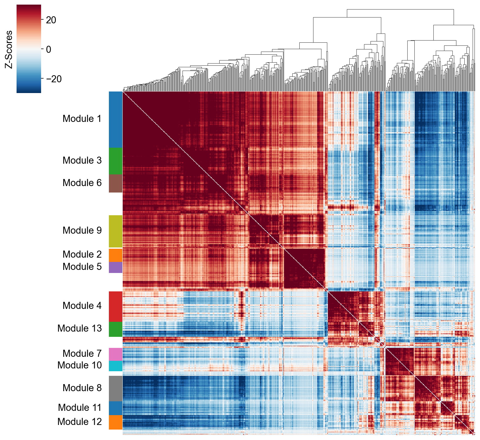
10 15
Name: count, dtype: int64
hs.plot_local_correlations(vmin=-30, vmax=30,)
<seaborn.matrix.ClusterGrid at 0x7f52ab7e3f10>
To explore individual genes, we can look at the genes with the top autocorrelation in a given module as these are likely the most informative.
# Show the top genes for a module

module = 4

results = hs.results.join(hs.modules)
results = results.loc[results.Module == module]

results.sort_values('Z', ascending=False).head(10)
| C | Z | Pval | FDR | Module | |
|---|---|---|---|---|---|
| Gene | |||||
| Btbd17 | 0.735443 | 221.872382 | 0.0 | 0.0 | 4.0 |
| Gadd45a | 0.666501 | 213.692549 | 0.0 | 0.0 | 4.0 |
| Neurog3 | 0.658402 | 208.855264 | 0.0 | 0.0 | 4.0 |
| Mdk | 0.695210 | 199.681646 | 0.0 | 0.0 | 4.0 |
| Tmsb4x | 0.628210 | 187.142300 | 0.0 | 0.0 | 4.0 |
| Neurod2 | 0.549973 | 183.843618 | 0.0 | 0.0 | 4.0 |
| Selm | 0.601179 | 178.700916 | 0.0 | 0.0 | 4.0 |
| Smarcd2 | 0.577830 | 174.089181 | 0.0 | 0.0 | 4.0 |
| Sox4 | 0.613079 | 173.945370 | 0.0 | 0.0 | 4.0 |
| Btg2 | 0.554990 | 165.342505 | 0.0 | 0.0 | 4.0 |
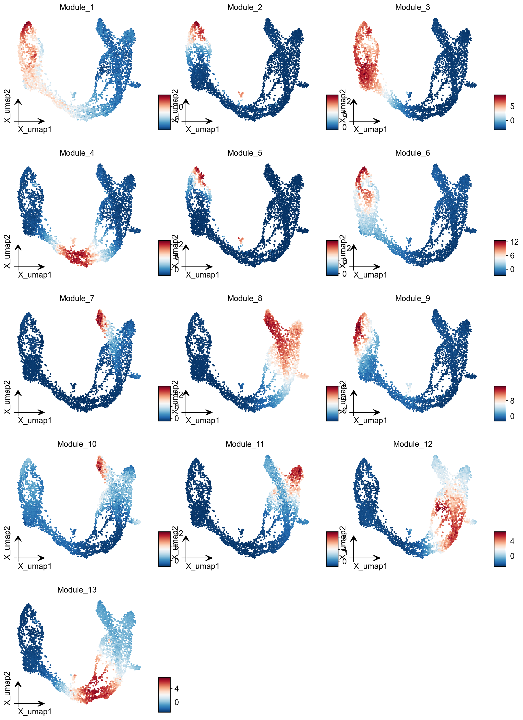
Summary Module Scores#
To aid in the recognition of the general behavior of a module, Hotspot can compute aggregate module scores.
module_scores = hs.calculate_module_scores()

module_scores.head()
Computing scores for 13 modules...
| 1 | 2 | 3 | 4 | 5 | 6 | 7 | 8 | 9 | 10 | 11 | 12 | 13 | |
|---|---|---|---|---|---|---|---|---|---|---|---|---|---|
| index | |||||||||||||
| AAACCTGAGAGGGATA | -6.583796 | -1.093584 | -3.131375 | -2.099180 | -0.819142 | -2.400016 | -0.451105 | 2.504838 | -2.298986 | -1.439230 | -0.739708 | 3.368700 | 0.531080 |
| AAACCTGAGCCTTGAT | 7.663903 | -0.765588 | 6.610663 | -2.388122 | -0.689135 | 2.296545 | -1.217827 | -3.391921 | 0.921212 | -0.813991 | -1.694216 | -2.358554 | -2.625691 |
| AAACCTGAGGCAATTA | -6.066218 | -1.212847 | -3.005648 | -2.684893 | -0.703958 | -2.226183 | -0.702572 | 2.636014 | -2.243965 | -0.119376 | 0.899747 | 2.736469 | -0.274772 |
| AAACCTGCATCATCCC | 11.594423 | 4.786089 | 5.015609 | -2.241397 | 0.848967 | 8.482152 | -0.886003 | -3.327994 | 12.943623 | 0.456323 | -1.689177 | -2.565122 | -2.858705 |
| AAACCTGGTAAGTGGC | -3.090054 | -1.036188 | -3.197947 | 5.563916 | -0.793746 | -2.413544 | -1.378844 | -2.149192 | -2.072845 | -2.134279 | -1.460957 | -0.137338 | 6.417286 |
module_cols = []
for c in module_scores.columns:
    key = f"Module_{c}"
    adata.obs[key] = module_scores[c]
    module_cols.append(key)
ov.pl.embedding(adata, basis='X_umap',color=module_cols,
           use_raw=False, ncols=3, frameon='small')
Fast NMF via nmf-rs (Rust port + 2024 SOTA algorithms)#
nmf-rs is a Rust port of
R’s NMF package plus modern algorithms (HALS, E-HALS Ang-Gillis 2019,
dnmf = DeBruine 2024 RcppML-style diagonalised NMF). It’s exposed
in omicverse as ov.single.NMF and gives ~75-280× speedup over R
on single-cell data, with comparable-or-better factor quality.
Recipes:
Recommended default:
method='dnmf'+ NNDSVD init, 25 iters → fastest configuration with strong biological signal (ARI ≈ 0.85 vs cell-type labels on PBMC 8k); diagonalised W·diag(d)·H removes scale ambiguity so L1 regularisation is meaningful.Strict R-reproduction:
method='lee'/'brunet'/'snmf/r'/ etc. — bit-equivalent to RNMF::nmf(...)within f64 round-off.Largest atlases (>500k cells):
dnmfkeeps NNDSVD warm-start + cache-friendly Rust kernels; ~30s on 200k cells × 5k genes.
Install: pip install nmf-rs. The wrapper imports it lazily so
omicverse keeps loading even without the optional dependency.
Initialise the NMF object#
Pass the same adata you preprocessed for cNMF. We use the
log-normalised counts (NMF requires non-negative input — NOT scaled
or PCA data).
rust_nmf = ov.single.NMF(adata, rank=12, use_hvg=True, num_threads=8)
rust_nmf
<omicverse.single.NMF rank=12 method=None init=None fitted=False>
Pick K via Brunet-style stability + reconstruction (cNMF-equivalent)#
Brunet et al. 2004 rank-selection philosophy: for each candidate K, run NMF many times with different random seeds and check both how stable the factorisation is across runs (consensus dispersion / silhouette) and how well it fits the data (reconstruction loss). Recommended K = biggest stability with reconstruction already plateaued.
This mirrors cnmf_obj.k_selection_plot() in the cNMF section above.
import time
t0 = time.perf_counter()
k_df = rust_nmf.select_k_brunet(
    np.arange(5, 16),
    method='dnmf',
    n_runs=30,
    max_iter=50,
)
print(f'K-selection runtime: {time.perf_counter() - t0:.1f}s')
print(f'auto-detected K: {rust_nmf.auto_k}')
k_df.round(4)
K-selection runtime: 129.8s
auto-detected K: 8
| rank | mean_loss | silhouette | |
|---|---|---|---|
| 0 | 5 | 7.185131e+06 | 0.7064 |
| 1 | 6 | 7.071660e+06 | 0.6999 |
| 2 | 7 | 6.977966e+06 | 0.6289 |
| 3 | 8 | 6.902006e+06 | 0.6602 |
| 4 | 9 | 6.858552e+06 | 0.5886 |
| 5 | 10 | 6.816046e+06 | 0.5628 |
| 6 | 11 | 6.789474e+06 | 0.5418 |
| 7 | 12 | 6.760640e+06 | 0.5228 |
| 8 | 13 | 6.736333e+06 | 0.4864 |
| 9 | 14 | 6.713335e+06 | 0.4632 |
| 10 | 15 | 6.692638e+06 | 0.4663 |
fig, ax = plt.subplots(figsize=(6, 3.2))
rust_nmf.k_selection_plot(ax=ax)
<Axes: title={'center': 'cNMF-style K selection — pick the K with peak silhouette'}, xlabel='rank (K)', ylabel='silhouette (higher = better)'>
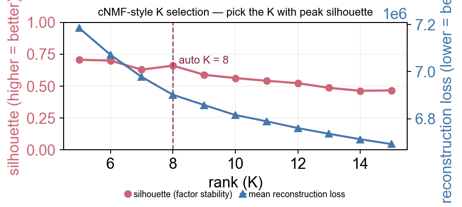
Reading the plot: silhouette (red, left axis) measures how reproducibly random initialisations land on the same K factor clusters across runs — higher = more stable. Reconstruction loss (blue, right axis) is the fit quality — lower = better fit.
The dashed purple line marks the auto-detected K via the stability-drop heuristic: K just before the largest drop in silhouette, gated by a plateau (or rise) coming into K. This combines two well-cited NMF rank-selection ideas:
Brunet et al. PNAS 2004 — pick K just before consensus stability drops sharply. Originally on cophenetic correlation; here we use the factor silhouette as a closely-related but more robust statistic.
Kim-Park 2007 — prefer K at a local maximum of the stability profile, not just the global peak (the global peak is usually the smallest K, the coarsest decomposition).
The heuristic falls back to the largest local peak when no plateau-drop
pattern exists (e.g. monotonic curves on tougher datasets) — in that
case bump n_runs and / or use method='brunet' for sharper signal.
Fit the recommended recipe (dnmf + NNDSVD)#
method='dnmf' (RcppML-style 2024) is fast and yields stable
diagonalised factors; NNDSVD init reduces initial loss by ~5 orders
of magnitude vs random runif, so 25 iterations are plenty.
selected_K = rust_nmf.auto_k     # Brunet+Kim-Park heuristic
print(f'Using auto-detected K = {selected_K}')

# Re-initialise with the chosen rank — the original NMF object was created
# with rank=12 as a placeholder; for the actual fit we use auto_k.
rust_nmf = ov.single.NMF(adata, rank=selected_K, use_hvg=True, num_threads=8)
Using auto-detected K = 8
%%time
rust_nmf.fit(method='dnmf', init='nndsvd', max_iter=25)
rust_nmf
CPU times: user 7.57 s, sys: 3.03 s, total: 10.6 s
Wall time: 911 ms
<omicverse.single.NMF rank=8 method=dnmf init=nndsvd fitted=True>
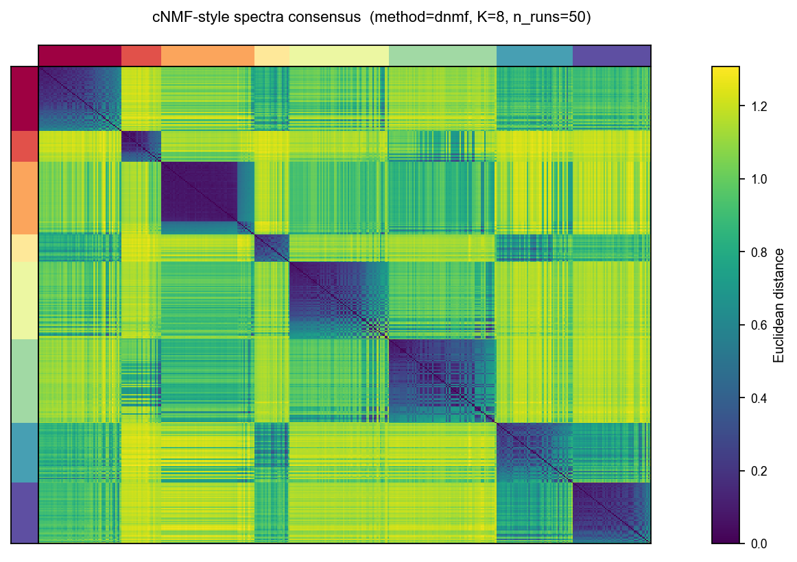
Brunet-style consensus heatmap#
Run NMF many times with different random seeds, average the binary
co-cluster matrices into a consensus C̄, and re-order both axes by
average-linkage hierarchical clustering of 1 - C̄. A perfectly
stable factorisation → K solid red diagonal blocks; instability →
smeared edges. Same idea as cnmf_obj.consensus(...) plot above.
rust_nmf.consensus(
    n_runs=50,         # 50 random inits — enough to see the K-block structure
    method='dnmf',
    max_iter=25,
)
rust_nmf.plot_consensus_heatmap(figsize=(6, 5))
<Axes: >
Push results into adata#
get_results adds the column-normalised cell usages to
adata.obsm['NMF_usage'], gene loadings to adata.varm['NMF_genes'],
and an argmax-over-factors module assignment to adata.obs['NMF_module'].
Returns a dict with usage_norm / gep_scores / top_genes —
same keys as cNMF’s result_dict for drop-in use.
result_dict = rust_nmf.get_results(adata, key_added='NMF', n_top_genes=30)
result_dict['usage_norm'].head()
| factor_1 | factor_2 | factor_3 | factor_4 | factor_5 | factor_6 | factor_7 | factor_8 | |
|---|---|---|---|---|---|---|---|---|
| index | ||||||||
| AAACCTGAGAGGGATA | 5.364271e-02 | 2.959199e-01 | 6.695385e-02 | 6.920532e-12 | 7.172111e-02 | 4.073585e-02 | 2.651638e-02 | 0.444510 |
| AAACCTGAGCCTTGAT | 1.692784e-01 | 7.774337e-12 | 7.854047e-12 | 4.798905e-01 | 7.784228e-12 | 7.837109e-12 | 1.857397e-01 | 0.165091 |
| AAACCTGAGGCAATTA | 4.571038e-02 | 2.509980e-01 | 1.609489e-01 | 2.316702e-02 | 7.264499e-12 | 4.187484e-02 | 5.947651e-02 | 0.417824 |
| AAACCTGCATCATCCC | 7.649092e-12 | 7.604145e-12 | 9.675541e-03 | 5.745508e-01 | 7.372807e-03 | 1.980603e-01 | 7.624490e-12 | 0.210341 |
| AAACCTGGTAAGTGGC | 1.076060e-01 | 1.224804e-01 | 6.978450e-12 | 5.621537e-03 | 2.875044e-01 | 6.963400e-12 | 6.926107e-12 | 0.476788 |
result_dict['top_genes'].head(5)
| factor_1 | factor_2 | factor_3 | factor_4 | factor_5 | factor_6 | factor_7 | factor_8 | |
|---|---|---|---|---|---|---|---|---|
| 0 | Ttr | Chga | Iapp | Spp1 | Btbd17 | Birc5 | Rps14 | Rps14 |
| 1 | Spp1 | Chgb | Pyy | Atp1b1 | Neurog3 | 2810417H13Rik | Malat1 | Rpl18a |
| 2 | Clu | Cryba2 | Pcsk2 | Cldn3 | Gadd45a | Cdca8 | Eef1a1 | Rps5 |
| 3 | Sparc | Cpe | Tmem27 | Mt1 | Cck | Cdca3 | Rpl18a | Rpl13a |
| 4 | Rpl18a | Pcsk1n | Rbp4 | Bicc1 | Tubb3 | Spc24 | Rpl10 | Eef1a1 |
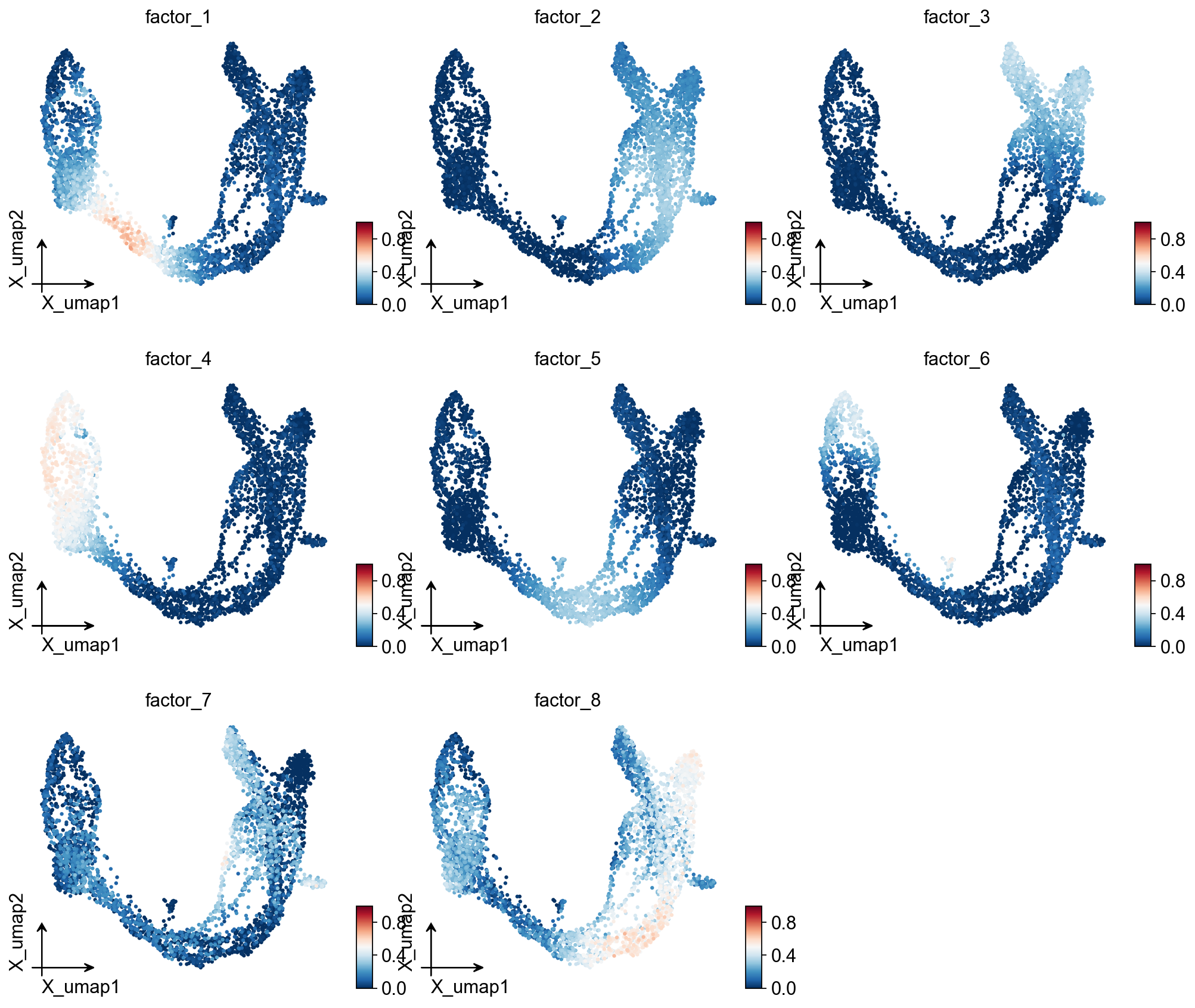
Visualise factor usages on UMAP#
ov.pl.embedding(
    adata, basis='X_umap',
    color=list(result_dict['usage_norm'].columns),
    use_raw=False, ncols=3, vmin=0, vmax=1, frameon='small',
)
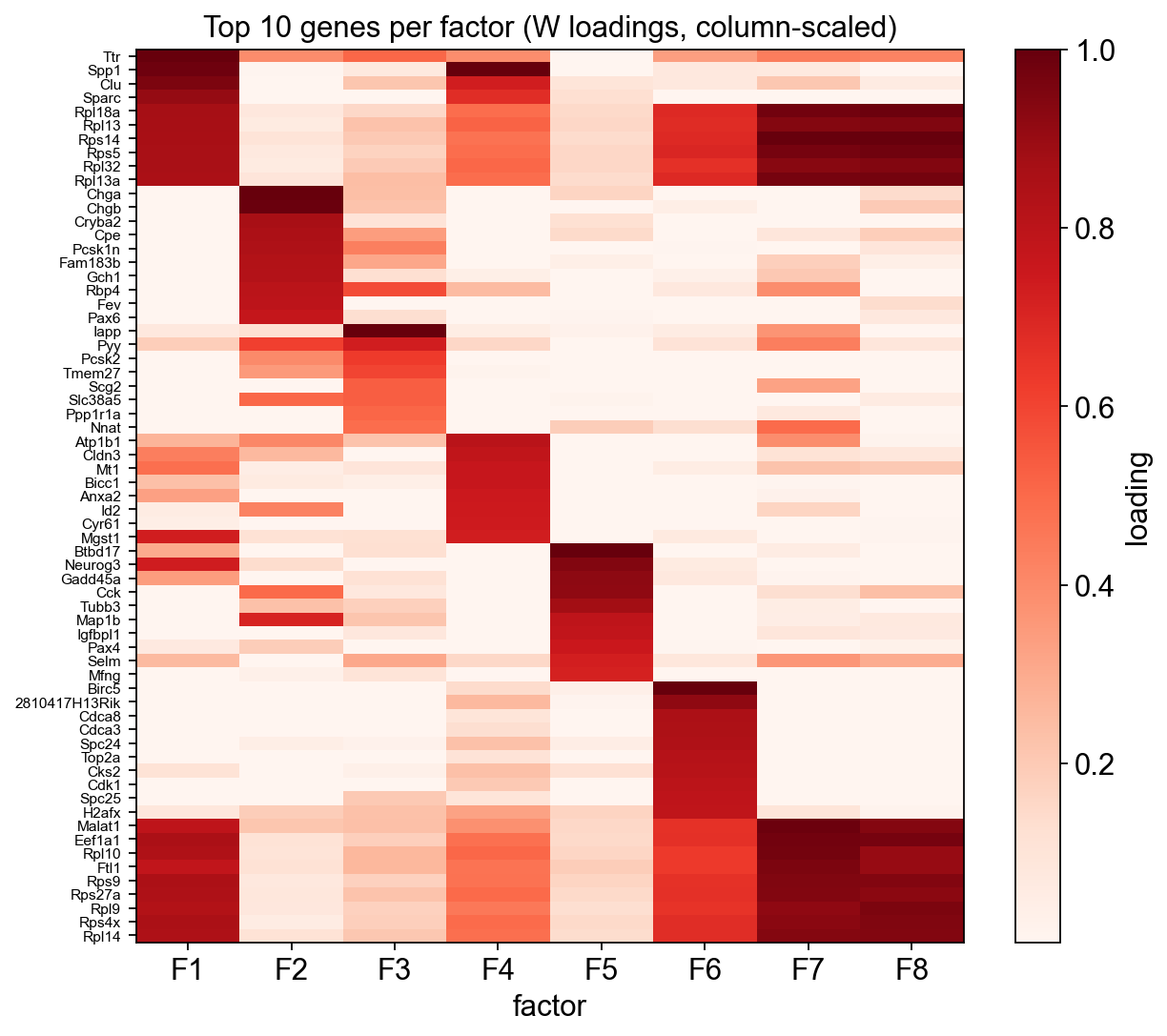
Top genes per factor (heatmap)#
ax = rust_nmf.plot_top_genes(n_top=10, figsize=(8, 7))
Random-forest module assignment (cNMF-style)#
Cells with a single dominant factor (max usage > threshold) seed an
RFC trained on PCA embeddings; the trained model is then applied to
ambiguous cells. Same idea as cnmf_obj.get_results_rfc.
rust_nmf.get_results_rfc(
    adata, result_dict,
    use_rep='scaled|original|X_pca',
    threshold=0.3, key_added='NMF_module_rfc',
)
RandomForestClassifier(n_jobs=-1, random_state=0)In a Jupyter environment, please rerun this cell to show the HTML representation or trust the notebook.
On GitHub, the HTML representation is unable to render, please try loading this page with nbviewer.org.
Parameters
| n_estimators | 100 | |
| criterion | 'gini' | |
| max_depth | None | |
| min_samples_split | 2 | |
| min_samples_leaf | 1 | |
| min_weight_fraction_leaf | 0.0 | |
| max_features | 'sqrt' | |
| max_leaf_nodes | None | |
| min_impurity_decrease | 0.0 | |
| bootstrap | True | |
| oob_score | False | |
| n_jobs | -1 | |
| random_state | 0 | |
| verbose | 0 | |
| warm_start | False | |
| class_weight | None | |
| ccp_alpha | 0.0 | |
| max_samples | None | |
| monotonic_cst | None |
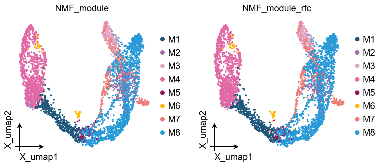
ov.pl.embedding(
    adata, basis='X_umap',
    color=['NMF_module', 'NMF_module_rfc'],
    frameon='small', legend_fontsize=14, legend_fontoutline=2,
    add_outline=False, outline_color='black', outline_width=1,
    show=False,
)
[<Axes: title={'center': 'NMF_module'}, xlabel='X_umap1', ylabel='X_umap2'>,
 <Axes: title={'center': 'NMF_module_rfc'}, xlabel='X_umap1', ylabel='X_umap2'>]
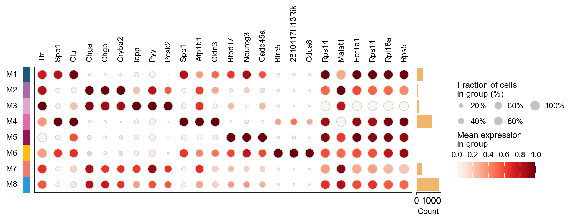
Dot plot of top genes per module#
plot_genes = []
for c in result_dict['top_genes'].columns:
    plot_genes += result_dict['top_genes'][c][:3].values.reshape(-1).tolist()
ov.pl.dotplot(
    adata, plot_genes, 'NMF_module_rfc',
    dendrogram=False, standard_scale='var',
)
<marsilea.heatmap.SizedHeatmap at 0x7f52c03e3f40>
When to pick which method?#
Use case |
Recommended |
Why |
|---|---|---|
Single-cell exploratory (default) |
|
Fastest with strong biology + stable diagonalised factors |
Strict R |
|
bit-eq R within 1e-12 |
Highest ARI vs cell-type labels (PBMC 8k benchmark) |
|
0.89 ARI vs 0.85 for dnmf — and bit-eq R |
Sparse factors + bit-eq R |
|
FCNNLS port + L1² regularisation |
Missing-value imputation |
|
weight=0 drops entries from loss |
See the rust-NMF repo for comprehensive benchmarks across small/medium/large dataset scales, factor-quality metrics (cophenetic, dispersion, Hoyer, ARI, Amari), and per-algorithm comparison vs cNMF and sklearn.