Single-cell copy-number variation with CopyKAT

This tutorial walks through ov.single.CNV(method='copykat') — a thin omicverse wrapper around the pure-Python py-CopyKAT re-implementation of the R CopyKAT method (Gao et al., Nature Biotechnology 2021).

CopyKAT is unsupervised: it classifies each cell as aneuploid (tumour) or diploid (normal) without needing a reference cell-type annotation. The wrapper writes results to a unified schema shared with inferCNV so the plotting helpers (ov.pl.cnv_heatmap, ov.pl.cnv_summary, ov.pl.cnv_umap) work with either backend.

Part.1 The math behind CopyKAT

CopyKAT runs an 11-step pipeline. The core ideas:

1. Stabilise raw counts. The variance-stabilising transform $\(\;\;y = \log(\sqrt{x} + \sqrt{x+1})\)$ maps Poisson-distributed counts to a near-Gaussian scale, after which the expression matrix is centred per cell.

2. Local denoising. A Kalman smoother sweeps along each chromosome to suppress per-gene noise while preserving step changes at copy-number breakpoints.

3. Baseline estimation. A Gaussian mixture (or the user-supplied norm_cell_names) identifies the diploid baseline, which is subtracted to give per-gene log-ratios.

4. Segmentation. A Poisson-gamma MCMC scheme detects breakpoints shared across cells, then aggregates genes into ~220 kb bins.

5. Classification. A KS-test on the aggregated CN profile flags each cell as \(\mathrm{aneuploid}\) (\(\Delta \mathrm{KS}\ge\tau\), default 0.1) or \(\mathrm{diploid}\). Aneuploid cells are then clustered by dynamic tree cut to recover subclones.

Reference: Gao et al., Nat Biotechnol (2021).

Part.2 Load data

We use the Maynard et al. (2020) lung adenocarcinoma 3 000-cell scRNA-seq benchmark. The file already carries gene-coordinate metadata in adata.var (chromosome, start, end), which both CopyKAT and inferCNV expect.

import omicverse as ov
ov.plot_set()

🔬 Starting plot initialization...
🧬 Detecting GPU devices…
✅ NVIDIA CUDA GPUs detected: 1
    • [CUDA 0] NVIDIA H100 80GB HBM3
      Memory: 79.1 GB | Compute: 9.0

   ____            _     _    __                  
  / __ \____ ___  (_)___| |  / /__  _____________ 
 / / / / __ `__ \/ / ___/ | / / _ \/ ___/ ___/ _ \ 
/ /_/ / / / / / / / /__ | |/ /  __/ /  (__  )  __/ 
\____/_/ /_/ /_/_/\___/ |___/\___/_/  /____/\___/                                              

🔖 Version: 2.1.3rc1   📚 Tutorials: https://omicverse.readthedocs.io/
✅ plot_set complete.

import os
import scanpy as sc
import omicverse as ov

# Maynard et al. (2020) lung adenocarcinoma scRNA-seq — 3 000 cells, 55 556
# genes, gene coordinates already in adata.var. Bundled by infercnvpy.
DATA_URL = "https://github.com/icbi-lab/infercnvpy/releases/download/d0.1.0/maynard2020_3k.h5ad"
data_dir = "data/cnv"
os.makedirs(data_dir, exist_ok=True)
adata = sc.read(f"{data_dir}/maynard2020_3k.h5ad", backup_url=DATA_URL)
adata

AnnData object with n_obs × n_vars = 3000 × 55556
    obs: 'age', 'sex', 'sample', 'patient', 'cell_type'
    var: 'ensg', 'mito', 'n_cells_by_counts', 'mean_counts', 'pct_dropout_by_counts', 'total_counts', 'n_counts', 'chromosome', 'start', 'end', 'gene_id', 'gene_name'
    uns: 'cell_type_colors', 'neighbors', 'umap'
    obsm: 'X_scVI', 'X_umap'
    obsp: 'connectivities', 'distances'

# Quick look at cell-type composition. Epithelial cells are the
# candidate tumour population; immune/stromal cells (Macrophage, T cell,
# Fibroblast, ...) act as the diploid majority CopyKAT needs to anchor
# the baseline against.
adata.obs["cell_type"].value_counts().head(10)

cell_type
Epithelial cell     522
Macrophage          409
Fibroblast          308
T cell CD4          259
T cell CD8          246
Monocyte            227
Endothelial cell    148
Plasma cell         139
other               115
mDC                 106
Name: count, dtype: int64

Part.3 Run CopyKAT

ov.single.CNV(method='copykat') consumes raw counts directly. For the 3 000-cell input it finishes in ~1-2 minutes on CPU (pycopykat is a Numba-accelerated port; no R / no GPU required).

After cnv.run():

slot	content
adata.obsm['X_cnv']	cells × ~12 k 220 kb bins of log-CN
adata.uns['cnv']['chr_pos']	chromosome → starting-bin index
adata.obs['cnv_prediction']	'aneuploid' / 'diploid' / NaN
adata.obs['cnv_score']	per-cell mean abs(log-CN)

cnv = ov.single.CNV(adata, method='copykat', genome='hg20')
cnv.run(verbose=False)

<omicverse.single._cnv.CNV at 0x7f2d113aa680>

adata.obs["cnv_prediction"].value_counts(dropna=False)

cnv_prediction
diploid      2561
aneuploid     412
NaN            27
Name: count, dtype: int64

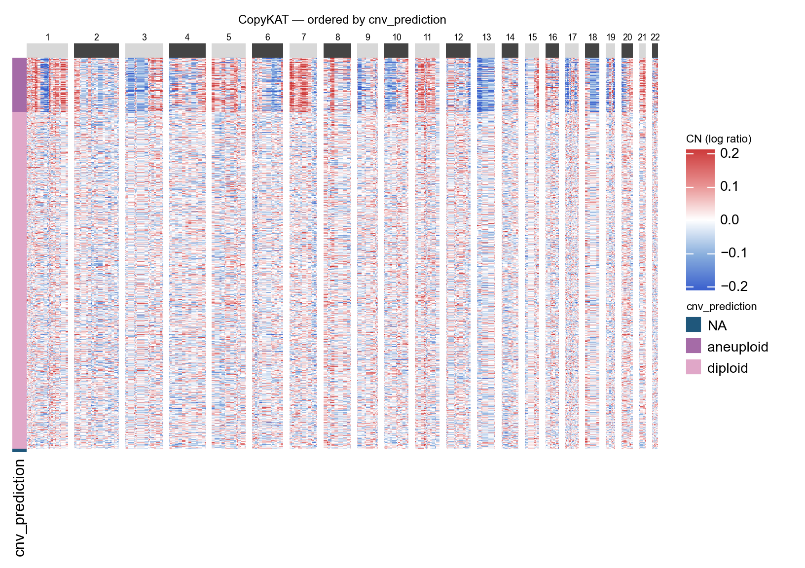
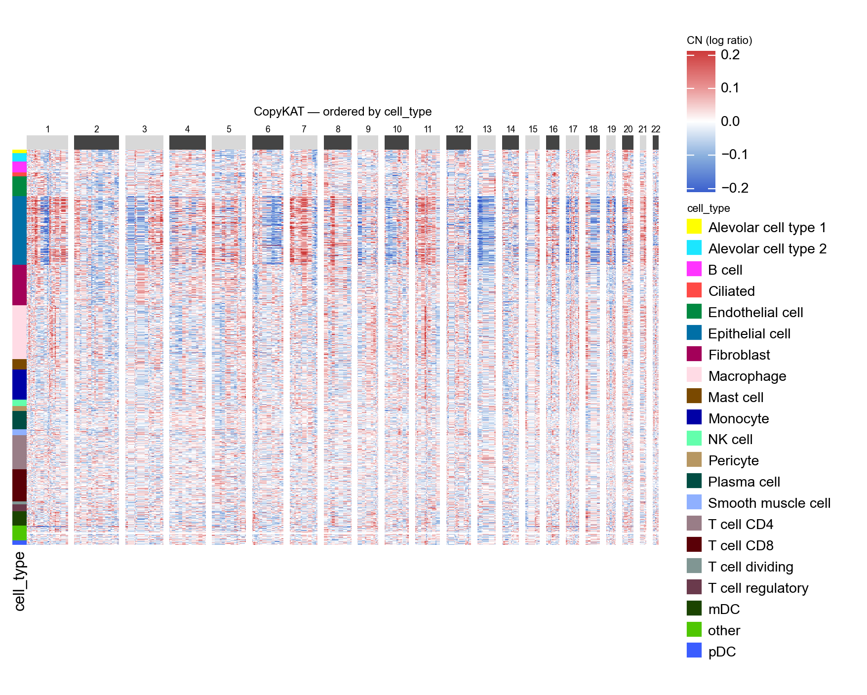
Part.4 Genome-wide heatmap

ov.pl.cnv_heatmap plots every cell as one row across the ordered genomic bins. Gain = red, loss = blue, with an alternating chromosome ideogram across the top. The groupby argument picks one adata.obs column to control row ordering and the group-divider lines. To compare cells under multiple labellings we draw two heatmaps — the same X_cnv matrix re-sorted by cnv_prediction and by cell_type — so we can read off whether the aneuploid band lines up with the Epithelial-cell cluster. Rendering uses marsilea for clean categorical legends (pass backend='matplotlib' to fall back to the pure-matplotlib renderer when marsilea isn’t installed).

# First view: ordered by the CopyKAT classification — aneuploid cells
# form a clean band at the top, diploid cells fill the rest.
ov.pl.cnv_heatmap(adata, groupby='cnv_prediction',
                  figsize=(8, 5), title='CopyKAT — ordered by cnv_prediction')

<marsilea.heatmap.Heatmap at 0x7f2d113aa470>

# Same matrix, re-ordered by cell_type. Recurrent CN patterns should
# concentrate inside the Epithelial-cell stripe.
ov.pl.cnv_heatmap(adata, groupby='cell_type',
                  figsize=(8, 5), title='CopyKAT — ordered by cell_type')

<marsilea.heatmap.Heatmap at 0x7f2f10384280>

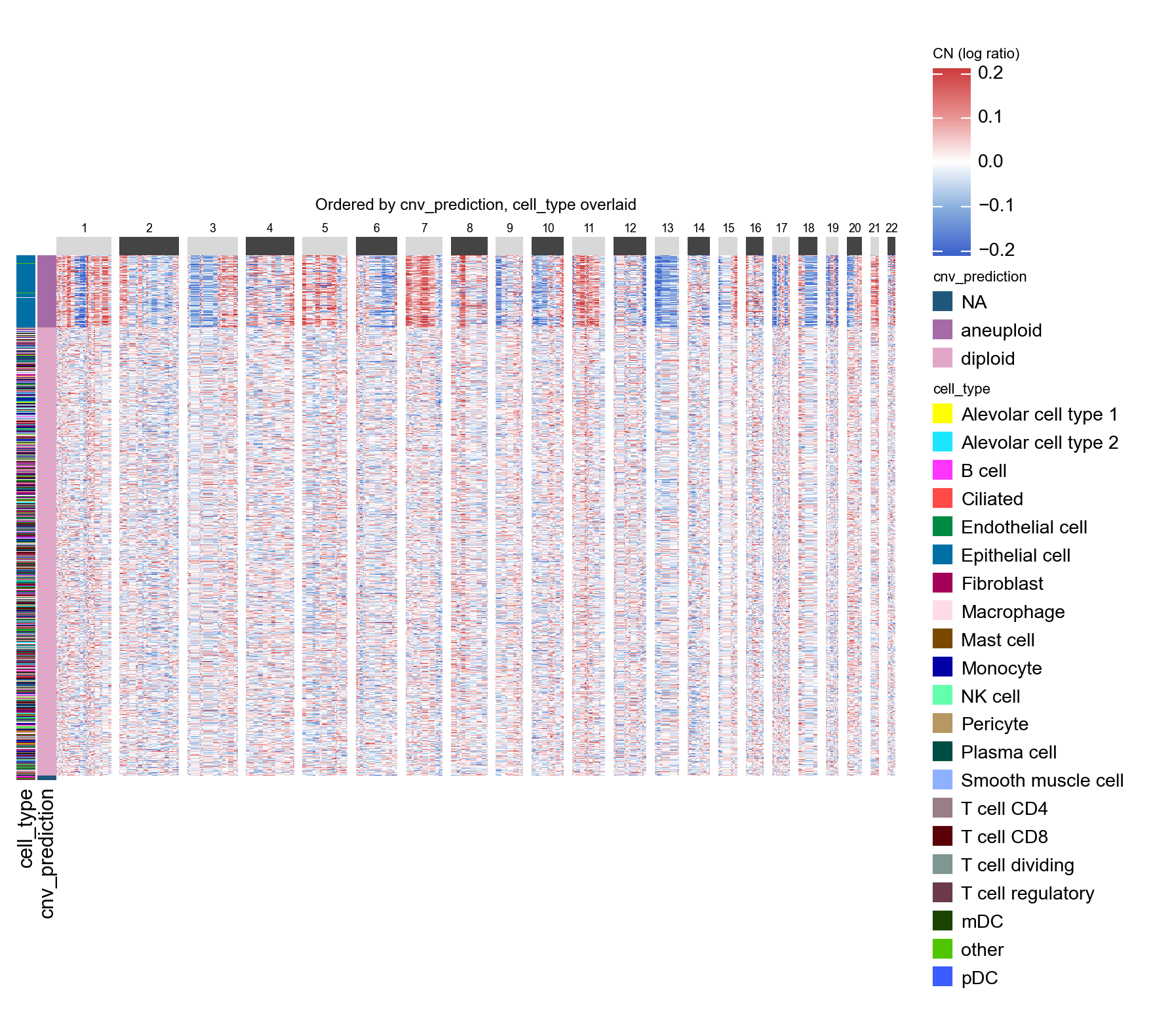
Layered annotation

If you want the row ordering of one column with an extra colour strip from another, pass the second column as annotations. The strip is purely decorative — it does not re-order cells, so you can see at a glance how a secondary category lines up against the primary grouping.

ov.pl.cnv_heatmap(adata, groupby='cnv_prediction', annotations=['cell_type'],
                  figsize=(8, 5),
                  title='Ordered by cnv_prediction, cell_type overlaid')

<marsilea.heatmap.Heatmap at 0x7f2ac7d222f0>

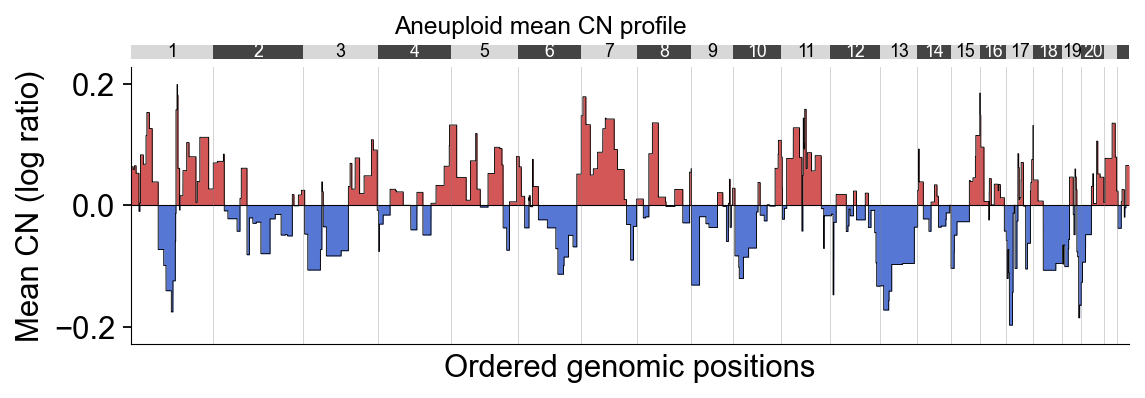
Part.5 Mean CN summary

ov.pl.cnv_summary reduces the heatmap to a single line: the mean log-CN across cells (or a subset) per genomic bin. Filling above zero (gain_color) and below zero (loss_color) makes copy-number gain / loss regions instantly visible. Below we plot the aneuploid mean — this is the de-facto pseudo-bulk CNV profile of the tumour.

ov.pl.cnv_summary(adata, groupby='cnv_prediction', subset='aneuploid',
                  figsize=(8, 2.6), title='Aneuploid mean CN profile')

(<Figure size 640x208 with 2 Axes>,
 {'line': <Axes: xlabel='Ordered genomic positions', ylabel='Mean CN (log ratio)'>,
  'ideogram': <Axes: >})

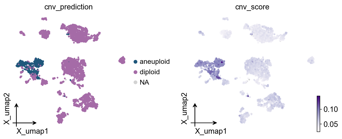
Part.6 UMAP

The dataset already has a UMAP in adata.obsm['X_umap']. ov.pl.cnv_umap colours it by the two columns CopyKAT writes — cnv_prediction (categorical) and cnv_score (continuous). The aneuploid cells should fall into one or a few coherent clusters that overlap with the original Epithelial-cell annotation.

ov.pl.cnv_umap(adata)

---

Next steps: for reference-anchored CNV inference (when you have a clean normal-cell annotation), see the inferCNV tutorial. For an in-depth comparison between CopyKAT and inferCNV on the same dataset, run both methods end-to-end and visualise their cnv_score columns side-by-side with ov.pl.embedding(adata, color=['cnv_score_copykat', 'cnv_score_infercnv']).