Lipidomics with LIPID MAPS and LION

Lipidomics data has distinctive structural properties that make a dedicated analysis path worthwhile:

• Features follow the LIPID MAPS shorthand ("PC 34:1", "TAG 54:3", "Cer d18:1/24:0") — you can extract lipid class + total carbons + total double bonds from the feature name alone

• Lipid classes (PC, PE, TAG, Cer, SM, …) are biologically-meaningful groupings — per-class totals often tell the story as clearly as per-species analysis

• The LION ontology (Molenaar et al. 2019, bioRxiv) groups lipid classes by shared biology (membrane vs storage, subcellular location, signalling role) and is the lipidomics analogue of GO for genes

This tutorial uses a real breast-cancer tissue lipidomics dataset from the lipidr R package (Mohamed et al. 2020, Bioinformatics): 20 patient samples × 412 lipid species, Cancer vs Benign. Every step below is on real published data — no synthetic spike-ins.

Covered:

1. parse_lipid — decode LIPID MAPS shorthand into structured fields

2. annotate_lipids — stamp class / carbons / double-bonds on adata.var

3. aggregate_by_class — collapse the per-species matrix to class-level totals

4. lion_enrichment — over-representation against the LION ontology

5. Standard univariate + multivariate pipeline on the lipid matrix

6. When to analyze at species-level vs class-level

import matplotlib.pyplot as plt
import numpy as np
import pandas as pd
import anndata as ad

import omicverse as ov

ov.plot_set()

🔬 Starting plot initialization...
🧬 Detecting GPU devices…
✅ NVIDIA CUDA GPUs detected: 1
    • [CUDA 0] NVIDIA H100 80GB HBM3
      Memory: 79.1 GB | Compute: 9.0

   ____            _     _    __                  
  / __ \____ ___  (_)___| |  / /__  _____________ 
 / / / / __ `__ \/ / ___/ | / / _ \/ ___/ ___/ _ \ 
/ /_/ / / / / / / / /__ | |/ /  __/ /  (__  )  __/ 
\____/_/ /_/ /_/_/\___/ |___/\___/_/  /____/\___/                                              

🔖 Version: 2.1.2rc1   📚 Tutorials: https://omicverse.readthedocs.io/
✅ plot_set complete.

1 — Download the dataset

The lipidr package ships two files in its inst/extdata/:

• brca_matrix.csv — 412 lipid species × 20 samples (features-in-rows)

• brca_clin.csv — sample-level clinical metadata (SampleType, Race, Stage, Tumor.Type)

Both live on GitHub (MIT-licensed) so we can pull them directly with ov.datasets.download_data. Total size: ~100 KB each.

matrix_path = ov.datasets.download_data(
    url='https://raw.githubusercontent.com/ahmohamed/lipidr/master/inst/extdata/brca_matrix.csv',
    file_path='brca_matrix.csv', dir='./metabol_data',
)
clin_path = ov.datasets.download_data(
    url='https://raw.githubusercontent.com/ahmohamed/lipidr/master/inst/extdata/brca_clin.csv',
    file_path='brca_clin.csv', dir='./metabol_data',
)

🔍 Downloading data to ./metabol_data/brca_matrix.csv
✅ Download completed
🔍 Downloading data to ./metabol_data/brca_clin.csv
✅ Download completed

2 — Load into AnnData

The layout is features-in-rows (412 lipids × 20 samples), so we transpose and join the clinical table on the sample ID. We also drop the 2 Metastasis samples to get a clean two-group comparison — Cancer (n=8) vs Benign (n=10).

The matrix is intensity-normalized (data comes from Purwaha et al. 2018, already log2-ish scaled by lipidr). We treat it as normalized concentration and skip PQN.

mat = pd.read_csv(matrix_path, index_col=0)      # 412 × 20, features-in-rows
clin = pd.read_csv(clin_path).set_index('Sample')

# transpose to samples-in-rows; align clinical metadata
X_df = mat.T                                       # 20 × 412
adata = ad.AnnData(
    X=X_df.to_numpy(dtype=np.float64),
    obs=clin.loc[X_df.index].copy(),
    var=pd.DataFrame(index=X_df.columns),
)
# Drop Metastasis for a clean 2-group comparison
adata = adata[adata.obs['SampleType'].isin(['Cancer', 'Benign'])].copy()
adata.obs['group'] = adata.obs['SampleType'].astype(str)
print(adata)
print('group split:', adata.obs['group'].value_counts().to_dict())
print('first 5 lipids:', list(adata.var_names[:5]))

AnnData object with n_obs × n_vars = 18 × 413
    obs: 'SampleType', 'Race', 'Stage', 'Tumor.Type', 'group'
group split: {'Benign': 10, 'Cancer': 8}
first 5 lipids: ['CE 16:0', 'CE 16:1', 'CE 18:0', 'CE 18:1', 'CE 18:2']

3 — Parse LIPID MAPS shorthand

ov.metabol.parse_lipid(name) decodes a single LIPID MAPS shorthand string. It returns a LipidIdentity dataclass with lipid_class, total_carbons, total_db, backbone, and raw. If the string doesn’t look like a lipid, the function returns None — so downstream code can filter or annotate.

Shorthand rules (abbreviated)

Shorthand	Components	Example
<CLASS> <C>:<DB>	sum-composition level — class, total carbons, total double bonds	PC 34:1 (PC, 34 C, 1 DB)
<CLASS> <backbone>/<C>:<DB>	sphingolipids — sphingosine (or variant) backbone + N-acyl	Cer d18:1/24:0 (Cer, d18:1 sphingosine, C24 saturated acyl)

Lipid classes the parser understands are in ov.metabol.LIPID_CLASSES (extensible). Glycerophospholipids (PC, PE, PS, PG, PI, PA, BMP + their lyso-forms), sphingolipids (SM, Cer + glyco-forms), neutral lipids (TAG, DAG, MAG, CE), and fatty acids are all covered.

# Demonstrate on a few canonical examples + some brca entries
for name in ['PC 34:1', 'TAG 54:3', 'Cer d18:1/24:0', 'LPC 18:0',
             adata.var_names[0], adata.var_names[200]]:
    lid = ov.metabol.parse_lipid(name)
    print(f'  {name:25s} → {lid}')

PC 34:1                   → LipidIdentity(lipid_class='PC', total_carbons=34, total_db=1, backbone=None, raw='PC 34:1')
  TAG 54:3                  → LipidIdentity(lipid_class='TAG', total_carbons=54, total_db=3, backbone=None, raw='TAG 54:3')
  Cer d18:1/24:0            → LipidIdentity(lipid_class='CER', total_carbons=24, total_db=0, backbone='d18:1', raw='Cer d18:1/24:0')
  LPC 18:0                  → LipidIdentity(lipid_class='LPC', total_carbons=18, total_db=0, backbone=None, raw='LPC 18:0')
  CE 16:0                   → LipidIdentity(lipid_class='CE', total_carbons=16, total_db=0, backbone=None, raw='CE 16:0')
  PC 16:1/24:1              → LipidIdentity(lipid_class='PC', total_carbons=16, total_db=1, backbone=None, raw='PC 16:1/24:1')

4 — Annotate the full matrix

ov.metabol.annotate_lipids(adata) applies parse_lipid to every adata.var_name and writes four new columns to adata.var:

Column	Type	Meaning
lipid_class	str	e.g. "PC", "TAG", "CER", None for unparseable
total_carbons	float	sum of acyl-chain carbons (nan if unparseable)
total_db	float	total double bonds
lipid_backbone	str	"d18:1" for ceramides, else None

The function returns a copy, not in-place, so the original is preserved for comparison.

adata = ov.metabol.annotate_lipids(adata)
print('class distribution:')
print(adata.var['lipid_class'].value_counts())
print(f'\nunparseable rows: {adata.var["lipid_class"].isna().sum()}')

class distribution:
lipid_class
PC    172
TG    155
DG     59
CE      8
PA      3
Name: count, dtype: int64

unparseable rows: 16

19 unparseable lipids — those are exotic species (plasmenyl-PC, plasmenyl-PE) that use a slightly different shorthand the parser doesn’t cover yet. You could extend LIPID_CLASSES or drop them for class-level analysis; we’ll drop them below.

5 — Class-level aggregation

A common first-pass view of lipidomics data is per-class total intensity: does the tumor have more total TAG than the benign controls? More total PC? aggregate_by_class(adata, agg='sum') collapses the n_species × n_samples matrix into a n_classes × n_samples one, with the default aggregation being the sum across species.

Aggregation options:

agg=	What it computes	When to use
"sum"	per-sample sum of all species in a class	“total PC abundance” — most common
"mean"	per-sample mean	normalize for class size, useful when classes have very different member counts
"median"	per-sample median	robust to outlier species

class_adata = ov.metabol.aggregate_by_class(adata, agg='sum')
class_adata.obs = adata.obs          # propagate clinical metadata
print('class-level matrix:', class_adata.shape)
print('\nclass → n_species:')
print(class_adata.var)

class-level matrix: (18, 5)

class → n_species:
    n_species
CE          8
DG         59
PA          3
PC        172
TG        155

# Quick per-class stacked-bar by group — the first plot every lipidomics paper shows
import seaborn as sns

df = pd.DataFrame(class_adata.X, index=class_adata.obs_names, columns=class_adata.var_names)
df['group'] = class_adata.obs['group'].values
df_long = df.groupby('group').mean().T
df_pct = df_long.div(df_long.sum(axis=0), axis=1) * 100

fig, ax = plt.subplots(figsize=(5, 4))
df_pct.T.plot(kind='bar', stacked=True, ax=ax, colormap='tab20', width=0.6)
ax.set_ylabel('% of total lipid intensity')
ax.set_xlabel('group')
ax.legend(loc='center left', bbox_to_anchor=(1.01, 0.5), frameon=False, fontsize=8)
ax.set_title('Lipid-class composition by group')
plt.tight_layout(); plt.show()

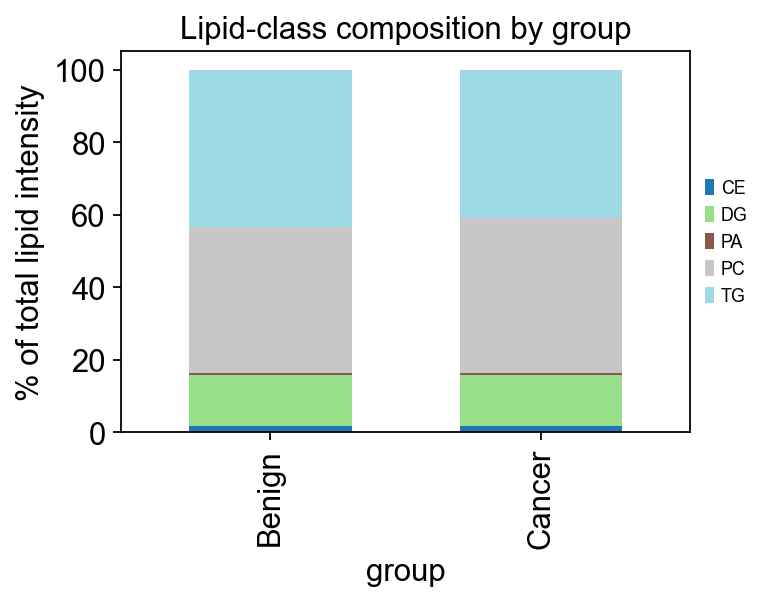
On brca the main class-level signal visible from this plot is a shift in TAG / CE balance between tumor and benign — consistent with the published Purwaha 2018 finding that tumor tissue has altered neutral-lipid storage.

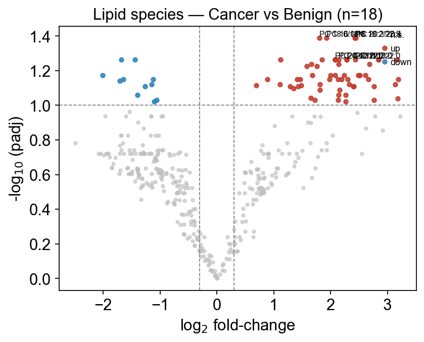
6 — Species-level differential + volcano

Now we run per-species differential analysis — same machinery as notebook 1, on the lipid matrix.

# Drop unparseable species and re-run on the clean matrix
adata_clean = adata[:, adata.var['lipid_class'].notna()].copy()
print('clean matrix:', adata_clean.shape)

# Data is already log-scaled by lipidr, so we use log_transformed=True
deg = ov.metabol.differential(
    adata_clean, group_col='group',
    group_a='Cancer', group_b='Benign',
    method='welch_t', log_transformed=True,
)
print(f'significant at padj<0.05: {(deg.padj<0.05).sum()}')
print(f'significant at padj<0.10: {(deg.padj<0.10).sum()}')

fig, ax = ov.metabol.volcano(deg, padj_thresh=0.10, log2fc_thresh=0.3, label_top_n=8)
ax.set_title(f'Lipid species — Cancer vs Benign (n={adata_clean.n_obs})')
plt.tight_layout(); plt.show()

clean matrix: (18, 397)
significant at padj<0.05: 4
significant at padj<0.10: 69

7 — LION ontology enrichment

LION (LIpid Ontology, Molenaar 2019) organizes lipid classes into categories:

• Class — which chemical family (Glycerophospholipids, Sphingolipids, Neutral lipids, Fatty acids)

• Function — biological role (Membrane constituents, Energy storage, Signalling lipids)

• Subcellular — predominant localization (Plasma membrane outer/inner leaflet, Mitochondrial, ER)

ov.metabol.lion_enrichment(hits, background) runs Fisher’s-exact ORA of these terms against a hit list. By default it calls ov.metabol.fetch_lion_associations() which downloads the full ~150-term LION ontology from GitHub (martijnmolenaar/lipidontology.com, ~14 MB) on first use and caches it at ~/.cache/omicverse/metabol/. Pass your own ontology= dict for domain-specific ontologies or to stay offline.

Parameters

Argument	Meaning
hits	lipid names in LIPID MAPS shorthand
background	all tested lipids
ontology	override the local LION subset (dict)
min_size	skip terms with fewer overlapping classes in the background

hits = deg[deg.padj < 0.10].index.tolist()
background = deg.index.tolist()
print(f'{len(hits)} differential lipid species at padj<0.10')

lion = ov.metabol.lion_enrichment(hits, background, min_size=2)
if lion.empty:
    print('no LION terms reached min_size — relax padj threshold')
else:
    lion.head(10)[['term', 'category', 'overlap', 'set_size',
                   'odds_ratio', 'pvalue', 'padj']]

69 differential lipid species at padj<0.10

8 — When to analyze species-level vs class-level

A common confusion in lipidomics papers: whether to report at the species level (PC 34:1) or class level (PC). Short answer — do both, and use them for different questions:

Question	Level	Reason
“Is total PC up or down in tumor?”	class	sums absorb per-species noise; enough power with small n
“Which specific lipid species drives separation?”	species	OPLS-DA VIP + S-plot; report single-species
“Does membrane / storage / signalling partition shift?”	LION term	aggregates across functional roles, not just chemistry

In a paper you would typically show all three: per-class stacked bar (Figure 2), species volcano (Figure 3), LION enrichment (Figure 4 — or a ridgeplot of the top LION terms’ effect sizes).

Summary

Step	Function	Notes
Parse name	ov.metabol.parse_lipid	returns None for unrecognized shorthand
Annotate matrix	ov.metabol.annotate_lipids	adds 4 cols to adata.var
Collapse to class	ov.metabol.aggregate_by_class	agg="sum" / "mean" / "median"
Species differential	ov.metabol.differential	same machinery as targeted metabolomics
LION enrichment	ov.metabol.lion_enrichment	category = class / function / subcellular

What’s not in this v0.2 lipidomics path (roadmap for v0.3)

• linex2-style lipid reaction network (requires shipping the reaction table; needs a license review)

• Saturation/carbon-number heatmaps (heatmap by class × (carbons, DB)) — easy to build on top of annotate_lipids, PR welcome

• LipidBlast / LipidSearch identification — that’s an upstream step, same as mzML → peak table

• Sphingolipid-specific tools (sphingosine headgroup deconvolution)