Spatial clustering with STAGATE + pymclustR#
STAGATE is a graph-attention auto-encoder. Bonus: it also produces a denoised expression matrix for downstream marker analysis.
This notebook runs the STAGATE spatial embedder on the
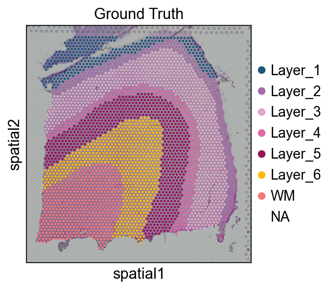
Maynard 151676 dorsolateral prefrontal cortex Visium sample
(3 460 spots × 10 747 genes) and clusters the resulting embedding with
pymclustR, a pure-Python
re-implementation of CRAN mclust (no rpy2 / R dependency).
Pre-processed input lives at
/scratch/users/steorra/analysis/omicverse_dev/omicverse-test/notebooks/data/cluster_svg.h5ad, which is the canonical fixture used in the originalt_cluster_spacetutorial.
0. Load AnnData + Ground Truth#
import omicverse as ov
import scanpy as sc
import pandas as pd, os, anndata as ad

ov.style(font_path='Arial')

# Load the pre-processed AnnData (3460 spots × 10747 genes — the same
# input the original spatial-clustering tutorial was developed against).
DATA_DIR = '/scratch/users/steorra/analysis/omicverse_dev/omicverse-test/data/151676'
H5AD     = '/scratch/users/steorra/analysis/omicverse_dev/omicverse-test/notebooks/data/cluster_svg.h5ad'
adata = ad.read_h5ad(H5AD)
truth = pd.read_csv(os.path.join(DATA_DIR, '151676_truth.txt'),
                    sep='\t', header=None, index_col=0)
truth.columns = ['Ground Truth']
adata.obs['Ground Truth'] = truth['Ground Truth'].reindex(adata.obs_names)
print('shape:', adata.shape, '  annotated:',
      adata.obs['Ground Truth'].notna().sum())
adata
🔬 Starting plot initialization...
Using already downloaded Arial font from: /tmp/omicverse_arial.ttf
Registered as: Arial
🧬 Detecting GPU devices…
✅ NVIDIA CUDA GPUs detected: 1
    • [CUDA 0] NVIDIA H100 80GB HBM3
      Memory: 79.1 GB | Compute: 9.0

   ____            _     _    __
  / __ \____ ___  (_)___| |  / /__  _____________
 / / / / __ `__ \/ / ___/ | / / _ \/ ___/ ___/ _ \
/ /_/ / / / / / / / /__ | |/ /  __/ /  (__  )  __/
\____/_/ /_/ /_/_/\___/ |___/\___/_/  /____/\___/

🔖 Version: 2.1.2rc1   📚 Tutorials: https://omicverse.readthedocs.io/
✅ plot_set complete.
shape: (3460, 10747)   annotated: 3431
AnnData object with n_obs × n_vars = 3460 × 10747
    obs: 'in_tissue', 'array_row', 'array_col', 'n_genes_by_counts', 'log1p_n_genes_by_counts', 'total_counts', 'log1p_total_counts', 'pct_counts_in_top_50_genes', 'pct_counts_in_top_100_genes', 'pct_counts_in_top_200_genes', 'pct_counts_in_top_500_genes', 'Ground Truth'
    var: 'gene_ids', 'feature_types', 'genome', 'n_cells_by_counts', 'mean_counts', 'log1p_mean_counts', 'pct_dropout_by_counts', 'total_counts', 'log1p_total_counts', 'space_variable_features', 'highly_variable'
    uns: 'REFERENCE_MANU', 'spatial'
    obsm: 'spatial'
    layers: 'counts'
sc.pl.spatial(adata, img_key='hires', color=['Ground Truth'])
1. Embed with STAGATE#
STAGATE (Dong & Zhang, Nat. Comm. 2022) is a graph-attention auto-encoder that combines spatial neighbourhood structure with gene expression. Adaptive edge weights let it capture local heterogeneity even at tissue boundaries.
methods_kwargs = {'STAGATE': {
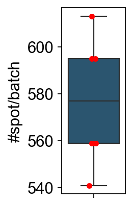
'num_batch_x': 3, 'num_batch_y': 2,
'spatial_key': ['X', 'Y'], 'rad_cutoff': 200,
'num_epoch': 1000, 'lr': 0.001,
'weight_decay': 1e-4, 'hidden_dims': [512, 30],
'device': 'cuda:0',
}}
adata = ov.space.clusters(adata, methods=['STAGATE'],
methods_kwargs=methods_kwargs)
The STAGATE method is used to cluster the spatial data.
------Calculating spatial graph...
The graph contains 3060 edges, 559 cells.
5.4741 neighbors per cell on average.
------Calculating spatial graph...
The graph contains 3328 edges, 595 cells.
5.5933 neighbors per cell on average.
------Calculating spatial graph...
The graph contains 3448 edges, 613 cells.
5.6248 neighbors per cell on average.
------Calculating spatial graph...
The graph contains 3044 edges, 541 cells.
5.6266 neighbors per cell on average.
------Calculating spatial graph...
The graph contains 3128 edges, 559 cells.
5.5957 neighbors per cell on average.
------Calculating spatial graph...
The graph contains 3320 edges, 595 cells.
5.5798 neighbors per cell on average.
------Calculating spatial graph...
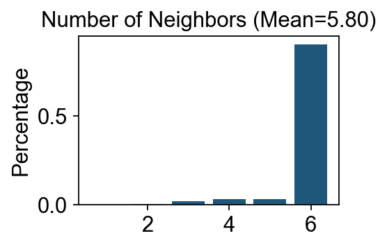
The graph contains 20052 edges, 3460 cells.
5.7954 neighbors per cell on average.
The STAGATE representation values are stored in adata.obsm["STAGATE"].
The rex values are stored in adata.layers["STAGATE_ReX"].
The STAGATE embedding are stored in adata.obsm["STAGATE"].
Shape: (3460, 30)
2. Cluster with pymclustR (no rpy2 / R needed)#
ov.utils.cluster(adata, use_rep='STAGATE', method='pymclustR',
n_components=10, modelNames='EEE', random_state=112)
adata.obs['pymclustR_STAGATE'] = ov.utils.refine_label(adata, radius=30, key='pymclustR')
adata.obs['pymclustR_STAGATE'] = adata.obs['pymclustR_STAGATE'].astype('category')
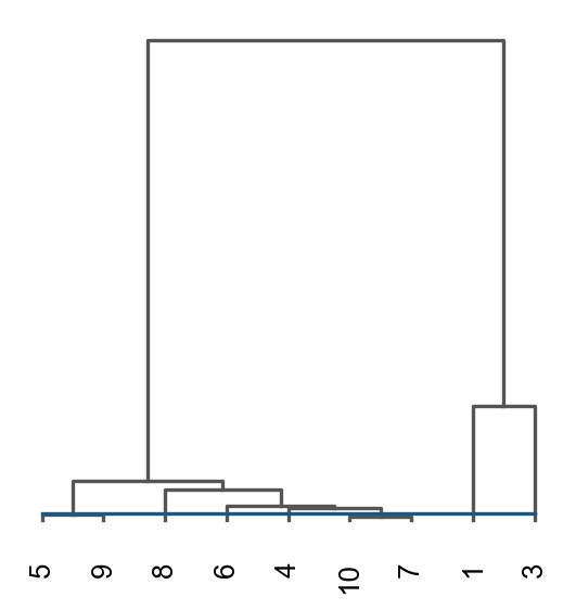
res = ov.space.merge_cluster(adata, groupby='pymclustR_STAGATE',
use_rep='STAGATE',
threshold=0.005, plot=True)
finished: found 10 clusters and added
    'pymclustR', the cluster labels (adata.obs, categorical)
    [model=EEE, loglik=-215474.7011, BIC=-437256.7467]
The merged cluster information is stored in adata.obs["pymclustR_STAGATE_tree"].
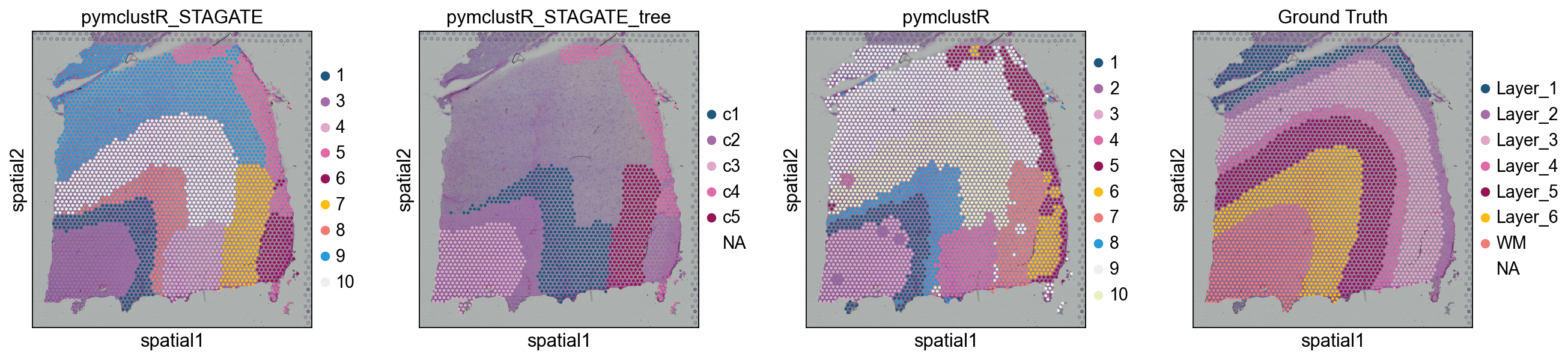
3. Spatial visualisation#
sc.pl.spatial(adata, color=['pymclustR_STAGATE',
                            'pymclustR_STAGATE_tree' if 'pymclustR_STAGATE_tree' in adata.obs.columns else 'pymclustR_STAGATE',
                            'pymclustR', 'Ground Truth'])
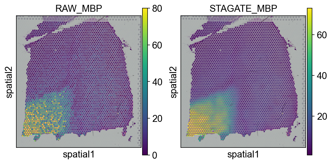
4. STAGATE denoising — reconstructed expression#
STAGATE also produces a denoised reconstruction in
adata.layers['STAGATE_ReX'].
import matplotlib.pyplot as plt
plot_gene = 'MBP'  # myelin marker — sharply enriched in white matter (WM)
fig, axs = plt.subplots(1, 2, figsize=(8, 4))
sc.pl.spatial(adata, img_key='hires', color=plot_gene, show=False,
              ax=axs[0], title='RAW_'+plot_gene, vmax='p99')
sc.pl.spatial(adata, img_key='hires', color=plot_gene, show=False,
              ax=axs[1], title='STAGATE_'+plot_gene, layer='STAGATE_ReX', vmax='p99')
[<Axes: title={'center': 'STAGATE_MBP'}, xlabel='spatial1', ylabel='spatial2'>]
5. ARI vs Maynard ground truth#
from sklearn.metrics.cluster import adjusted_rand_score

obs = adata.obs.dropna(subset=['Ground Truth'])
ari_raw = adjusted_rand_score(obs['pymclustR'], obs['Ground Truth'])
ari_ref = adjusted_rand_score(obs['pymclustR_STAGATE'], obs['Ground Truth'])
print(f'STAGATE + pymclustR (raw):     ARI = {ari_raw:.4f}')
print(f'STAGATE + pymclustR (refined): ARI = {ari_ref:.4f}')
STAGATE + pymclustR (raw):     ARI = 0.3692
STAGATE + pymclustR (refined): ARI = 0.3756